Learning Outcomes: Upon completion of this lab, you will gain practical experience in: 

• Calculating concentrations and amounts
• Pipetting accurately and precisely 
• Solution making
• Amplifying DNA
• Setting-up a polymerase chain reaction experiment

This lab focuses on pipetting basics and PCR amplification of the E. coli folA gene. 

• In Part A, pipetting basics, you will learn how to use micropipettes with accuracy and precision. You will also learn the basics of solution making. 
• In Part B of this lab, you will design PCR primers (refer to the chapter “Think Tank 2” in Teaching Resources) and test these primers in your PCR. Your instructor will also design and optimize a set of primers that will be used as a positive control to PCR amplify your folA gene. You should always keep in mind why you are conducting this experiment. This step marks the beginning of your research project towards expressing, purifying, and characterizing your protein of interest; DHFR (Dihydrofolate Reductase). 

 This experimental plan is possible due to many scientific discoveries, some of which include: 

1. Recombinant DNA cloning by Stanley Norman Cohen (and others) in 1973 (1). 

2. Restriction endonucleases (aka. restriction enzymes) by Warner Arber, Daniel Nathans, and Hamilton Smith (2-7). These two discoveries led to the production of insulin, a true Canadian connection (8). 

3. Discovery of PCR (Polymerase Chain Reaction) by Kari Mullis in 1983 (9-10). Other discoveries also helped build this field of Recombinant DNA Cloning (11). 

4. Another great example is the identification of a bacterial plasmid by Joshua Lederberg in 1953 (Profiles in Science: The Joshua Lederberg Papers) (12).

Background information – Part A: Laboratory Basics: Pipetting and Preparing Solutions

Use of Pipettors

In Part A of this lab you will learn how to use a pipettor (also known as a micropipettor or pipette) to accurately measure and dispense small volumes of liquid. Pipettors are a common piece of equipment in a biochemistry lab and thus competence (and confidence!) in using them is an essential skill.  You will have lots of practice using pipettors from this lab and throughout the course. 

Proper use of a pipette is instrumental in ensuring experimental success. The majority of molecular biology deals with small volumes (less than 1000 μL). For example, your PCR reaction volume is a whopping 50 μL! This means that you must pipette all your reagents (DNA template, primers, polymerase, dNTPs, and buffer) in exact volumes to ensure success for your PCR. Pipetting mistakes will change the concentration of your reagents and therefore can result in no PCR amplicon (fun fact: an amplicon refers to a fragment of DNA that is the result of an amplification procedure). In your case, the DNA fragment containing your folA gene is known as the amplicon in your reaction. Thus, you need to master the art of pipetting such that you are both accurate and precise in your execution, so what do these two terms mean? 

To calculate the accuracy (A) of our pipettes we can use the following equation:

These are units, but watch what you can do with these if you treat them like typical fractions and apply basic arithmetic rules:

Things to note:

Keep in mind the units you are using and make sure you undergo appropriate inter-conversions. Many different types of concentration measurements can only be inter-converted between one another if additional information is available. For example: to convert from mg/mL to mM you need to know the molecular weight of the solute.

Dilution – “is when one substance (often but not always water) is added to another to reduce the concentration of the first substance. The original substance being diluted may be called the stock solution.” (19) For example, a 1 in 10 (or 1/10) dilution of a stock solution in a final volume of 10 mL means that you add 1mL of your stock solution to 9 mL water. (19)

Stock solution – concentrated solution, which you dilute prior to use

Working solution – diluted solution, ready to use

Dilution factor – is a dimensionless number that unambiguously describes the strength of the dilution. It is equal to the volume of the stock solution used divided by the total volume of the working solution produced. The dilution factor also gives the relationship between solute concentration in the stock solution and the working solution. (19)

Serial dilution – A sequential set of dilutions in which the stock for each dilution in the series is the working solution from the previous dilution.

Background – Part B: PCR amplification of your E. coli folA gene

Polymerase Chain Reaction (PCR)

72°C – (Extension step) The thermostable DNA polymerase (such as Taq DNA polymerase) is now able to make copies of each strand starting from each annealed primer. This extension temperature can vary depending on the polymerase used.

Putting this whole process together, we obtain the following PCR diagram:

Figure 1 – Schematic diagram illustrating the concept of PCR. Image created by Felicia (loosely adapted from (22)

Please note that the unamplified, double-stranded DNA (containing your folA gene of interest) is first denatured (high heat) prior to the annealing of primers. The primers are complementary to each DNA strand and flank the beginning and end of your folA gene. The extension of the new DNA strand occurs from the free 3’ – OH end of each primer. Once annealed, the temperature is set for optimal extension of the primers to complete the new DNA strands. This step requires a thermostable DNA polymerase and dNTP’s (not shown in this figure). The cycle continues (denaturation, annealing, and extension) using the newly formed DNA strands as template DNA.

The Tm (melting temperature of primers) can be calculated for each primer using the following general formula:

The Tm of a pair of primers (forward and reverse) should be within a range of 1-4 degrees to ensure optimal PCR amplification. As a general rule-of-thumb, the Ta (annealing temperature of primers) is usually estimated to be 5 degrees below the Tm

These two equations are really important and you should commit them to memory. However, calculating annealing temperatures of primers is not solely dependent on the C/A/T/G composition, but also on the pH of the reaction, salts present, etc. These buffer conditions make a HUGE impact on the melting and annealing temperature. Nowadays, many companies that make and sell oligonucleotide primers also have their own, free primer annealing temperature calculators that mimic some of the real-world conditions in your reaction tube. It is important to keep in mind that these numbers are, at best, an educated guess to give you a starting point with respect to your first reaction conditions. Typically, when setting up PCR samples, you would test more than one condition to pinpoint the optimal reaction condition that yields a product. A couple of really good rules to follow are: 

• Always understand what you are doing – know what you need to add to each tube and why each reagent is there. 
• Always double-check that your primers are correct with respect to complementarity. Nowadays you can use many freeware computer programs for this task, but you can also ask a colleague to look over your gene sequence and your primer sequences to double, triple make sure. 
• Use a computer program to determine your annealing temperature and try to use a program supplied by the company you will be ordering your primers from. 
• Test more than one annealing temperature condition. 
• Use a checklist when adding reagents to a PCR tube in order to ensure that you’ve added everything in the tube. 
• Double, triple-check your reagents and the proper concentrations you need to add for each reagent.

Please click on this link to learn about pipetting basics: Pipetting basics

The following table is a guide depicting the pipetting range of each type of micropipette. You should NEVER exceed the upper or lower limits of these pipettors. 

Some examples are provided below (1):

Figure 2: Volume setting examples. Figure adapted from the Gilson guide to pipetting (1)

2. Place a tip on the discharge end of the pipettor. Note: If sterile conditions are necessary do not allow the pipet tip to touch any object (including your hands). Please do NOT place the pipette over your books.

Figure and excerpt adapted from: http://www.pipette.com/public/staticpages/guidetopipetting.aspx

” The plunger will stop at two different positions when it is depressed. The first of these stopping points is the point of initial resistance and is the level of depression that will result in the desired volume of solution being transferred. Because this first stopping point is dependent on the volume being transferred, the distance you have to push the plunger to reach the point of initial resistance will change depending on the volume being pipetted. The second stopping point can be found when the plunger is depressed beyond the initial resistance until it is in contact with the body of the pipettor. At this point, the plunger cannot be further depressed. This second stopping point is used for the complete discharging of solutions from the plastic tip. You should not reach this second stop when drawing liquid into the pipettor, only when expelling the last drop. Before continuing, practice depressing the plunger to each of these stopping points until you can easily distinguish between these points ” (15)

3. Press the plunger to the first stop (i.e. until you feel resistance) and then insert the tip of the pipette into the desired solution. Ensure that the tip is submerged in the solution, about 1/3 to halfway. Please do not submerge the pipette tip all the way to the bottom of the tube as this can create a seal between the tip and tube thereby resulting in the wrong volume pipetted. (15)

4. To allow the desired solution volume into the pipette tip you will need to slowly, and carefully, release the pipette plunger. If you remove your thumb pressure from the plunger too quickly it will yield an inaccurate volume. This is especially true if the solution being pipetted is more viscous than water. (15) 

5. Transfer the solution to an appropriate container/tube by inserting the tip into the tube. It is typically recommended that you angle the tip against the tube wall, or, if there is a solution already present in the tube, you submerge the tip in the solution prior to dispensing the liquid (though this is not always the case). To dispense the solution from the pipette tip simply depress the plunger (slowly) until you arrive at the first stop (first point of resistance). Stop here and wait for a second before continuing to the second stop. You can now slowly remove the tip from the solution. (15)

6. Discard the tip in the appropriate waste container by pressing down on the tip ejector on your pipette. Remember to change tips between solutions to avoid mixing or contaminating the solutions used. (15)

When carrying pipettes, never walk around with a pipette containing a sterile tip on it. It is not only a sharps hazard, but the tip is no longer sterile. Never hold the pipette upside down such that the liquid in the tip can enter the body of the pipette. Pipette tips are sterile and located in tip boxes. Be very gentle when opening the box and only keep the box open for the duration of time it takes you to add a fresh tip to the pipette. Keep tip boxes closed to maintain tip sterility.

Please click this hyperlink to access the Chapter 1 virtual lab bench

Please click this hyperlink to access the “Proper Handling of Pipette” video

Run through the “Using a micropipette” section outlined on how to use a micropipette. Make sure you are comfortable operating a pipette before continuing with the protocol.

Let’s recap our pipetting best practices by clicking in this video: Pipetting basics

Please click this hyperlink to access the Pipette “First Stop versus Second Stop” video

1. Practice delivering varying amounts of water using all the different micropipette sizes available at your lab station. Make sure the amount chosen is within the acceptable limits of the micropipette you are using. Please do NOT over-exceed the upper or lower limits of the pipette as it will damage the pipette. 

2. To confirm that the correct amount of liquid was delivered dispense the water onto a weigh boat and weigh the water on a balance.

The density of water is 1 g/mL, therefore: 

1 mL H₂O = 1 g 

Given the volume range of micropipettes, it would be best if we calculate the weight of 1 µL of water and work with this value. 

1 µL H₂O = 1×10^-3 g = 1 mg

3. Demonstrate, using a scale, that you can accurately pipette one volume (e.g. 7.5 µL, 17 µL, 99 µL, and 551 µL). Choose one pipette, take the pipette to the weigh scale (along with a tip box). Choose one volume and measure out each volume 5 times.  Record your measurements in the table provided and fill in the rest of the table in your notes. In the observations section discuss how accurate and precise your pipette is.

Following this pipetting protocol, we implement a SUPER FUN pipetting activity that we adapted from the “Pipetting by Design” lab (CPET University of Florida). The Word file containing the template designs can be found here (29).

The image below depicts a sample of our students’ pipetting results. This entire exercise requires micropipettes, food coloring, and 96-well plates, along with a design template (see Word file, above).

Before we begin amplifying our folA gene using Polymerase Chain Reaction (PCR), we first need to understand where this piece of our project fits in with the overall goal of molecular DNA cloning. So why does the first part of our research project begin with molecular DNA cloning? To incorporate the E. coli folA gene into a specific plasmid DNA! This plasmid DNA will allow us to express and purify our gene product: Dihydrofolate Reductase (DHFR) protein. This diagram depicts the overall workflow for chapters 1-5 of our course… but this is just an aerial view of this intricate process.

Now it is time to delve into the details of this workflow.

So what exactly is molecular DNA cloning? Well, let’s click on the following module to find out: Molecular cloning module

To recap, molecular DNA cloning refers to a set of techniques that allows us to manipulate DNA. For our course, the main goal is to clone the folA gene into a circular piece of DNA called a plasmid. This plasmid is unique because it allows us to introduce our gene of interest (aka. folA) into bacteria so we can then transcribe/translate the gene into its protein product: DHFR.

This workflow for manipulating DNA to yield pure protein can be applied to countless biochemistry research projects. And so, let’s look at our specific molecular cloning workflow:

Step 1: PCR-amplify the folA gene. Actually, before we even begin step 1 we need to design our primers. Students can work individually or in small groups to design one set of primers. Instructors should also take care to design and optimize a second set of primers which will serve as a positive control. The primers should flank our folA gene … but wait, there’s more. For this next part we need to have a strong understanding of our main goal (expression of our protein of interest) and ensure that we incorporate any necessary elements needed for this goal when we manipulate the DNA. Also, please remember that the PCR primers are DNA primers and become incorporated into the newly synthesized DNA strand during PCR. Why is this so cool? Because we have the ability to introduce new DNA at either end of the gene. This is exactly what we are going to do. We are going to add Restriction Enzyme (RE) recognition sites for 2 unique REs at either end of the folA gene by incorporating these RE recognition sites at the 5′ ends of each primer. In this way we have designed primers to PCR amplify our folA gene and we can manipulate this amplicon later using restriction enzymes!

Step 2: Restriction Enzyme (RE) digestion of the folA amplicon and pET26b plasmid using two unique restriction enzymes (RE-1 and RE-2).

This step allows us to generate restriction-enzyme-specific “sticky ends” which direct the insertion of the folA gene into the pET26b plasmid. We will learn a lot about these sticky ends in chapter 2 of this course.

This leads us to step 3:

Step 3: Insert the RE-digested folA gene into the RE-digested pET26b plasmid using the molecular glue known as DNA ligase.

And job done! Of course, we do need to check that we successfully cloned our folA gene into the pET26b plasmid. How? Why using Restriction Enzyme mapping and Sanger sequencing techniques!

It is now time to PCR amplify the folA gene. Please review “Part B: amplification of folA using PCR” chapter prior to tackling this protocol. 

Prior to this lab, we introduceour students (working alone or in small groups) to primer design by asking our students to collaborate together in one of our Team Think Tanks (refer specifically to Team Think Tank 2: Primer Design). If you wish to learn more about our Team Think Tanks, click here.

Please note, Instructors should also design and optimize  a second set of primers.

Before beginning this lab, 

You will use the PCR primers you designed in one reaction, and the PCR primers designed by your instructor in the second reaction.

Please click this hyperlink to access the Chapter 1 virtual lab bench

Please click this hyperlink to see how we set up the thermocycler (aka. PCR Machine)

Please click this hyperlink to see how we use the microspectrophotometer (aka. Nanodrop)

DNA can be quantified by measuring the absorbance at 260 nm using a spectrophotometer. This is a happy consequence of the fact that purines and pyrimidines have a conjugated double-bond system that absorb light in the ultraviolet spectrum (260 nm). There is a simple conversion formula used by scientists in the lab, which states that on average, an absorbance reading of 1 (i.e. 1 A₂₆₀) at 260 nm is ~ = to 50 µg/mL double-stranded DNA. 

Given this conversion factor, please calculate your working concentrations for the sample of template DNA, knowing that the sample was measured at 260nm. 

Reagents must be kept on ice. Prior to the start of your experiments acquire a bucket of ice. Discuss with your instructor how you will label your PCR tubes. Record your tube labels in your lab notebook. Please note, the PCR tube has a very small area for writing on the cap (do not write on the side of the tube as it will rub off when placed in the Thermocycler). 

You will be given the primers that you have designed and manufactured by a scientific company, primers will be lyophilized (i.e. freeze-dried so they appear in crystalline form). 

Please calculate the amount (µL) of nuclease-free water needed to re-suspend (i.e. dissolve the freeze-dried primer DNA into a solution) the lyophilized PCR primers to a final concentration of 100 µM each. 

Record pertinent information and calculations in your lab notebook.

1.  Add the calculated amount of nuclease-free water to each tube of lyophilized primers. Once added, vortex the tubes for 1-2 minutes (make sure you fasten the cap securely before you start to vortex your sample). 

2. Prepare a 1/10 dilution of each stock primer by taking 2 fresh, microcentrifuge tubes and labeling them appropriately as forward and reverse primers. 

For each primer, please dilute 1/10 from the stock primer tube into the fresh microcentrifuge; a total volume of 30 µL each. 

In your lab notebook answer the 2 questions.

1. How many µL of stock primer do you need to add to each tube? 

2. How many µL of water do you need to add to each tube (final volume = 30  uL)?

These 2 diluted primers will be used as your forward and reverse primers for one of your two reactions.

PCR components: 50 µL total volume

Copy the chart in your lab notebook and fill it in.

Practical lab considerations 

(Image created by Felicia, centrifuge obtained from Presenter Media © 2009-2021 Eclipse Digital Imaging, Inc.)

Once finished, please clean up your work area. Properly dispose of reagents properly and safely as specified by your lab mentor, and please wash your hands.

(1)Cohen, S. N.; Chang, A. C.; Boyer, H. W.; Helling, R. B. Construction of biologically functional bacterial plasmids in vitro. PNAS 1973, 70, 3240–3244. 

(2) Kresge, N.; Simoni, R. D.; Hill, R. L. The Characterization of Restriction Endonucleases: the Work of Hamilton Smith J. Biol. Chem. 2010, 285, e2-e3. 

(3) Kelly, S.; Kaddurah-Daouk, R.; Smith, H. O. Purification of the HhaII Restriction Endonuclease from an Overproducer Escherichia coli Clone J. Biol. Chem. 1985, 260, 15339–15344. 

(4) Kaddurah-Daouk, R.; Cho, P.; Smith, H. O. Catalytic Properties of the HhaII Restriction Endonuclease J. Biol. Chem. 1985, 260, 15345–15351. 

(5) Arber, W.; Linn, S. DNA modification and restriction. Ann. Rev. of Biochem. 1969, 38, 467–500. 

(6) Brownlee, C. Danna and Nathans: Restriction enzymes and the boon to molecular biology. Proc. Natl. Acad. Sci. U.S.A. 2005, 102, 5909. 

(7) Danna, K.; Nathans, D. Specific changes of simian virus 40 DNA by restriction endonuclease of Hemophilus influenzae. Proc. Natl. Acad. Sci. U.S.A. 1971, 68, 2913–2917. 

(8) Villa-Komaroff, L.; Efstratiadis, A.; Broome, S.; Lomedico, P.; Tizard, R.; Naber, S. P.; Chick, W. L.; Gilbert, W. A bacterial clone synthesizing proinsulin. Proc. Natl. Acad. Sci. U.S.A. 1978, 75, 3727–3731.

(9) Pray, L. The biotechnology revolution: PCR and the use of reverse transcriptase to clone expressed genes. Nature Education, 2008, 1, 1. 

(10) Mullis, K. B.; Faloona, F. A. Specific synthesis of DNA in vitro via a polymerase-catalyzed chain reaction. Meth. Enzym. 1987, 155, 335–350.

(11) DNA Technology Milestones collection. http://www.nature.com/milestones/miledna/pdf/miledna_all.pdf (accessed July 10, 2013). 

(12) Profiles in Science: The Joshua Lederberg Papers. http://profiles.nlm.nih.gov/BB/ (accessed July 10, 2013). 

(13) Boyer, R. Biochemistry Laboratory: Modern Theory and Techniques, 2nd ed.; Pearson Education Inc., 2012; pp. 309-324. 

(14) Taylor, J. R. An Introduction to Error Analysis: The Study of Uncertainties in Physical Measurements, 2nd ed.; University Science Books, 1999 pp. 128–129. 

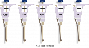
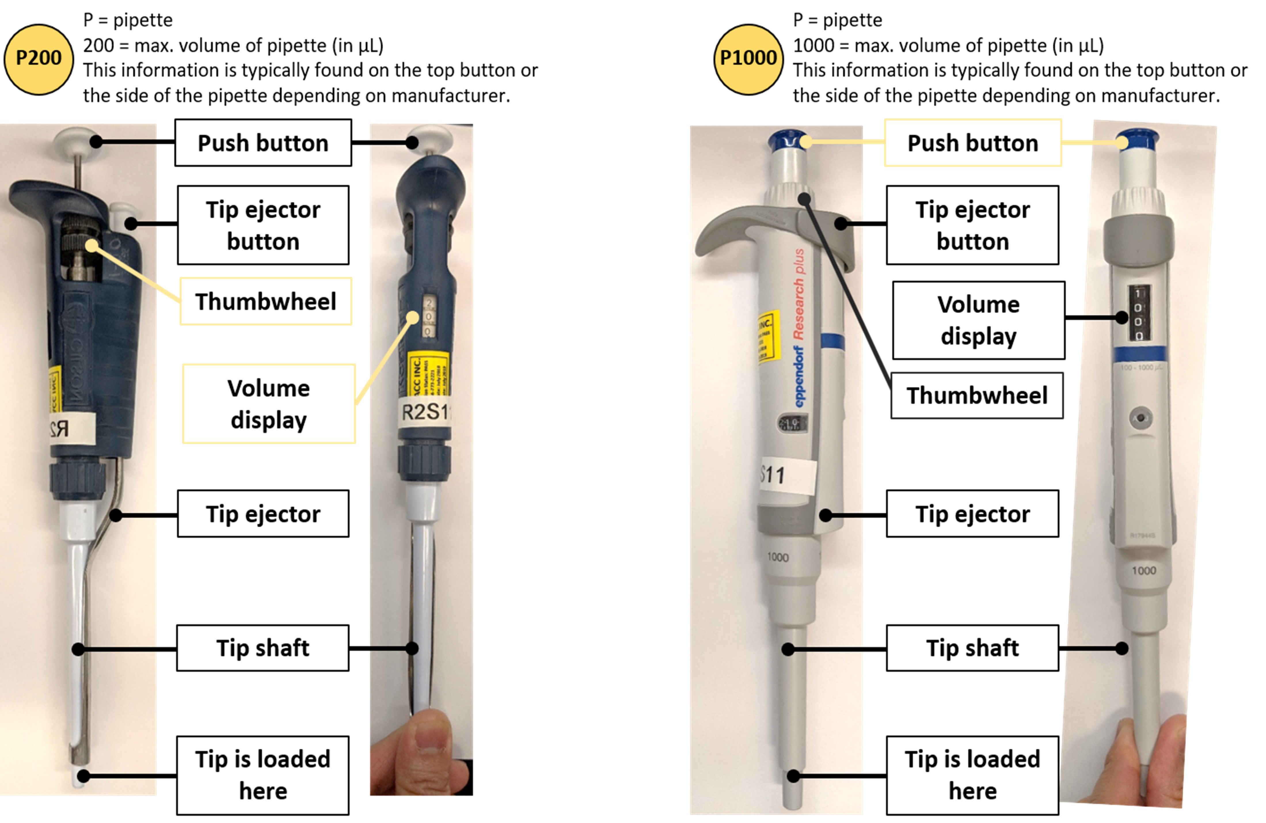
(15) Davidson College, Department of Biology, How to use a micropipettor. http://www.bio.davidson.edu/courses/Molbio/Protocols/pipette.html (accessed May 15, 2021), © Copyright 2002 Department of Biology, Davidson College, Davidson, NC 28036. 

(16) University of Regina, Department of Biology, proper use of pipetters. http://bio305lab.wikidot.com/appendix:pipettes (accessed May 15, 2021) 

(17) Reed, R.; Holmes, D.; Weyers, J.; Jones, A. Practical Skills in Biomolecular Sciences, 2nd edition.; Prentice Hall, 2003.

(18) Shakhashiri, Z. Chemical Demonstrations: A Handbook for Teachers of Chemistry. Volume 2; University of Wisconsin Press, 1985. 

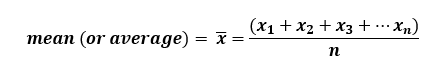
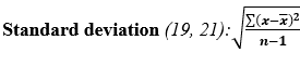
(19) Seidman, L. A. Basic Laboratory Calculations for Biotechnology, Pearson Education Inc.; 2008. 

(20) Voet, D.; Voet, J. D.; Pratt, C. Fundamentals of Biochemistry, 3rd ed.; John Wiley and sons Inc., 2008. 

(21) Standard deviation by Robert Niles. https://www.robertniles.com/stats/stdev.shtml (accessed May 15, 2021). 

(22) Newton, C.R.; Graham, A. PCR, 2nd edition.; BIOS Scientific Publishers, Oxford, 1997; pp. 1-27. 

(23) The Nobel Prize in Chemistry 1993, Nobelprize.org. 13 Jun 2013. http://www.nobelprize.org/nobel_prizes/chemistry/laureates/1993/ (accessed May 15, 2021)

(24) Glaser, J.A. Validity of Nucleic Acid Purities Monitored by 260 nm/280 nm Absorbance Ratios, BioTechniques, 1995, 18, 62-63. 

(25) Thein, S. L.; Wallace R. B. (1986). The use of synthetic oligonucleotides as specific hybridization probes in the diagnosis of genetic disorders. In Human genetic diseases: a practical approach, Davis, K. E.), IRL Press, Herndon, Virginia, 1986; p. 33-50. 

(26) Innis, M. A.; Gelfand, D. H.; Sninsky, J. J.; White, T. J. PCR protocols: a guide to methods and applications. Academic Press; 1990. 

(27) Lawyer, F. C.; Stoffel, S.; Saiki, R. K.; Myambo, K.; Drummond, R.; Gelfand, D. H. 1989. Isolation, characterization, and expression in Escherichia coli of the DNA polymerase gene from Thermus aquaticus. J. Biol. Chem.1989, 264: 6427-6437. 

(28) Pearson Custom Library; 2016 – “Making Decisions with Data” chapter obtained from the following book: Hage, D. S., & Carr, J. D. (2011). Analytical chemistry and quantitative analysis. Boston: Prentice Hall.

(29) Bokor, J. R., & Darwiche, H. (2011b, October). Pipetting by design. Paper presented at the annual conference of the National Association of Biology Teachers, Anaheim, CA.

Other references of interest:

a. McPherson, M. J.; Moller, S. G. PCR. BIOS Scientific Publishers Ltd., 2000; pp. 1-83. 

b. Suggs, S. V.; Wallace, R. B.; Hirose, T.; Kawashima, E. H.; Itakura, K. (1983) Use of synthetic oligonucleotides as hybridization probes: isolation of cloned cDNA sequences for human beta 2-microglobulin. Proc Natl Acad Sci U S A.1983, 78, 6613-6617. 

c. Eckert, K. A.; Kunkel, T. A. DNA polymerase fidelity and the polymerase chain reaction. Genome Res. 1991, 1, 17-24. 

d. Kolmodin, L.A.; Williams, J.F. Polymerase Chain Reaction: Basic Principles and Routine Practice, The Nucleic Acid Protocols Handbook; Humana Press, Totowa, New Jersey, 2000; pp. 569-580.

Learning Outcomes: Upon completion of this lab, students will gain practical experience in: 

• Working with restriction enzymes 
• Preparing an agarose gel and in loading DNA samples 
• Interpreting DNA gels

In this lab you will conduct the following workflow:

1. Check to see if your PCR was successful. How? Using agarose gel electrophoresis. You will load a small sample from your PCR tubes on an agarose gel, then your DNA bands will be separated based on size using the electrophoresis technique. You will also analyze the NdeI/XhoI digested pET26b plasmid as a control to ensure that the restriction enzymes are functional.

2. You have now PCR amplified your folA gene. Congratulations!!!! The PCR products containing your amplicons (amplicon: technical term for amplified or replicated nucleic acids) must now be digested with the 2 restriction enzymes (REs) you engineered in your primers as 5’ extensions: NdeI and XhoI.

This will create two distinct sticky ends, which will allow us to control the direction of inserting our folA gene into the pET26b plasmid. This process is referred to as directional cloning (1). These restriction enzymes are present in the pET26b (2) multiple cloning site and should position your folA gene in the proper orientation with respect to the T7 promoter. Remember that the 5’to 3’ gene sequence translates to the  N-terminal to C-terminal direction in a protein sequence. These samples will not be loaded on the agarose gel. We will store these samples until the next lab (chapter 3). 

Restriction Enzyme (RE) Basics

The discovery of restriction endonucleases (or, more simply, restriction enzymes) revolutionized molecular biology (3-6). Using these enzymes scientists can “cut”, or “digest”, DNA at specific sites. The sizes of the resulting DNA fragments can be determined, providing a map of the DNA. Importantly, under the right conditions, the DNA fragments that result from digestion with restriction endonucleases can be joined, or ligated, to other DNA fragments. Such recombination is the basis of a phrase used to describe a significant aspect of biochemistry and molecular biology: “recombinant DNA technology”. In this lab, you will learn how to recombine fragments generated by these enzymes (7).

Restriction enzymes are produced mainly by bacterial cells and are used to degrade various forms of DNA. This includes foreign DNA from bacteriophages, thus such endonucleases “restrict” entry of foreign DNA into a bacterial host. 

Restriction enzymes are useful for molecular cloning because they recognize specific sequences and cut double-stranded DNA. There are four main types of restriction enzymes available, but we will focus only on one basic type for this course: type II restriction enzymes.

For example, EcoRI is a restriction enzyme (RE) readily available for purchase from companies such as New England Biolabs (NEB) or Thermo Fisher Scientific. EcoRI recognizes a specific hexanucleotide sequence, G*AATTC, and the enzyme cleaves at the asterisk point (yellow arrowhead in the image).

One thing to note is that restriction enzymes recognize palindromic sequences, meaning that these sequences are the same on opposite strands when read in the 5’ to 3’ direction. In our EcoRI example to the left, GAATTC can be read on both DNA strands as long as you read each strand in the 5’ to 3’ direction. This is a unique feature that allows for specific cleavage of both DNA strands.

Also, note that the naming of restriction enzymes tells you a lot about where this enzyme initially came from. EcoRI can be broken down as follows: the first 3 letters abbreviate the organism source, in this case, Escherichia coli (E. coli); the next letter represents the strain, in this case the R strain of E. coli; the Roman numeral gives us insight into the order of discovery. In this case, EcoRI was the first restriction enzyme to be discovered from the R strain. Remember that in science the name of an organism, compound, enzyme, etc. contains a LOT of history so instead of memorizing names… look them up and see how they were derived!

Agarose Gel Electrophoresis

DNA is super small and not readily visible to the naked eye. As such, once we “cut” our DNA with restriction enzymes we will obtain a number of different DNA fragments. These fragments are typically different in size: some are short and some are long. However, since we cannot see DNA we cannot easily separate the different sized DNA pieces … or can we? Enter a cool technique called agarose gel electrophoresis. 

The main component of this technique is a slab of gel. That’s right, a gel. Though this gel is not made up of Jell-O, it is very similar in concept to Jell-O. You can actually look at a slab of Jell-O and a slab of agarose and you will note many similarities: both slabs are jelly-like substances that can be soft or firm depending on their temperature. Now the main ingredient in Jell-O is gelatin. The main ingredient in an agarose gel is agarose.

Schematic diagram of an agarose gel. Image created by Felicia.

Agarose is a linear polymer made up of the repeating unit of agarobiose: a disaccharide composed of alternating residues of D-galactose and 3,6-anhydro-L-galactopyranose. Agarose polymers create a meshwork through which DNA migrates when an electric field is applied. Because DNA has a negative charge it will migrate towards the positive pole in an electric field (electrophoresis). The agarose matrix serves as a “molecular sieve” that will separate larger DNA fragments from smaller fragments. 

There are several factors that influence the rate of migration of DNA through agarose gels. These are highlighted in the table below (adapted from Sambrook, 2001, page 5.4-5.7, (3)). 

In this lab, you will use agarose gel electrophoresis to visualize and analyze the results of your PCR amplification. You will prepare your own gels and gain experience in interpreting DNA gels.

In agarose gel electrophoresis, DNA is typically added into each well of a freshly prepared agarose gel slab.

Image created by Felicia. 

The agarose slab is placed in an electrophoresis tank which contains one negative and one positive electrode at either end of the gel. We can then take advantage of the overall negative charge character of the DNA backbone in order to separate DNA fragments of different sizes by applying a current running from negative to positive. DNA will readily migrate towards the positive end. The agarose matrix itself will function as a sieve to impede migration of DNA fragments of varying sizes. In this system, smaller DNA fragments migrate faster towards the positive electrode. 

However, DNA is not visible to the naked eye while an agarose gel is running.  Thus there we need to use other methods to monitor how electrophoresis is progressing.  To accomplish this, scientists typically add tracking dyes to their samples (the resulting dye has a blue appearance).  These dyes are visible to the naked eye and migrate through the gel in a manner similar to the DNA molecules.  The sample buffer that you will be using (see the “Materials” section later on) includes two tracking dyes: xylene cyanol FF and bromophenol blue.  While the migration rates of these dyes relative to the migration of DNA fragments of specific lengths varies with changes in the percentage of agarose in the gel, there is still a general correlation between dye migration and DNA migration.  For agarose gels between 0.7 and 1.7 % agarose; xylene cyanol, light blue color, migrates at approximately the same rate as a linear double-stranded piece of DNA that is ~ 4 kbp (kilobase pair) in length. Bromophenol blue, dark blue color, migrates at approximately the same rate as a DNA fragment that is ~ 300 bp long (3). 

To visualize the actual DNA bands in the gel, the DNA itself must be stained with a dye. In our case, you will be using GelRed which is added to the liquid form of the agarose gel right before it is poured into the gel casting tray. The dye itself will intercalate with DNA fragments and fluoresce when exposed to UV light. This is why it is very important to wear your UV-protective safety goggles when conducting this last step. In our lab we will be using a UV transilluminator which bypasses the need for us to look directly into the UV light. Instead, we will be visualizing the results using a camera and a laptop, however the UV light will still be employed in this process therefore safety measures must be followed at all times. Below are some examples of possible results.

Possible agarose gel results. DNA samples were digested with BamHI (B), EcoRI (E), HindIII (H) or no restriction enzyme (-) and run on an agarose gel. Gels were visualized following DNA staining.

Figures were adapted from Micklos, David A., and Greg A. Freyer. DNA science; a first course in recombinant DNA technology. Cold Spring Harbor Laboratory Press, 1990, pp. 274.

Centrifugation – in this lab you will also be using the technique of centrifugation to “pellet” your reaction. Throughout our experiments we will be employing this technique quite a bit, thus it is important to take a moment and understand its basic use. For this lab our only concern is ensuring that our different mixture components are thoroughly mixed and brought to the bottom of our microcentrifuge tube for easy access. In later labs we will be utilizing this technique to separate our bacterial cells from growth media, as well as other uses. 

Helping students understand how to determine DNA fragment sizes following RE digestion reactions makes for a great Team Think Tank. Please check out Team Think 3: Restriction Enzyme Digests located in the Teacher Resources section.  If you wish to learn more about our Team Think Tanks, click here.

What are your expected DNA band sizes? 

This question is actually quite complex and requires knowledge of the DNA sequence for both pET26b plasmid and the E. coli folA gene (and sequence of the DNA primers used in the PCR). OK, let’s unpack this, starting with the pET26b plasmid.

The pET26b plasmid sequence can be sourced from many locations. One such location is the AddGene portal: pET26b sequence

The sequence can be processed using molecular cloning software. There are many molecular cloning software programs available, and some are free to use. We recommend SnapGene. This is a paid software but it does have a basic, freeware version called SnapGene viewer.

This is a map generated from the actual pET26b DNA sequence. Note the different features of the plasmid and their base pair (bp) location on the plasmid. The pET26b plasmid is a circular, covalently-closed double-stranded DNA, 5360 bp in length.

The main features are:

• the T7/lac promoter – this is the main event! An inducible promoter (i.e. we control when this promoter is off or on). We are cloning our folA gene downstream of this promoter.
• NdeI and XhoI – the two Restriction Enzymes (RE) we are using to clone our folA gene downstream of the T7/lac promoter. Note the bp position in brackets beside each RE. This indicates the bp position of the cut site for each RE.
• His 6x-tag – this is an engineered tag consisting of the codon for the amino acid histidine repeated six times. Why? Because this His 6x-tag will be used later for protein purification.
• kanR gene, selectable marker – the kanamycin resistance gene is situated downstream of a constitutive promoter (i.e. always on) and is used as a selectable marker for bacterial transformations.
• Ori – the origin of replication for the pET26b plasmid
• lacI – a gene that expresses the Lac repressor, a protein used to control the T7/lac promoter.

And so, based on this map we can say the following:

Full length pET26b plasmid = 5360 bp

pET26b plasmid previously digested with NdeI and XhoI =? To answer this question let us zoom in on the pET26b plasmid map and look at the actual sequence surrounding the NdeI and XhoI restriction enzyme DNA recognition sites:

The yellow highlighted area contains the DNA fragment cleaved out following NdeI/XhoI digestion of the pET26b plasmid. We can count the number of base pairs (bp) in this area to determine the fragment size cleaved out of the plasmid. We typically report the base pair sizes relative to the sense strand (5’ to 3’) only. This is to standardize our reporting system, however, we need to keep in mind that we are cleaving both strands of the DNA using restriction enzymes NdeI and XhoI. If we count base pairs (using the bp numbers on the right as a guide) we can see that the NdeI cuts at exactly the 5070 bp position (remember, we report the bp position relative to the sense strand only). We can physically count the base pairs in the yellow highlighted area (there are 128 bps) before we reach the first “c” in the XhoI DNA recognition site, which cuts at exactly bp 5198. This process for determining DNA fragment sizes works well, but it is time-consuming. Instead, we can take a shortcut based on the information provided in the original, pET26b circular plasmid map shown above. The position of the restriction enzymes (NdeI and XhoI) relative to the T7/lac promoter is clearly indicated… but so are the base pair cut sites! Woohoo!!!!!! Note the numbers in brackets beside each restriction enzyme. These are the same bp positions as we determined using the actual sequence. Well now, this is just simple math. Let’s take a look using this basic diagram or our pET26b plasmid.

Upon successful cleavage of both strands of DNA using restriction enzymes NdeI and XhoI: We will obtain two, linear DNA fragments. Why two? Because we are cutting a circular, covalently closed piece of DNA. Based on this diagram, we obtain the following DNA fragments following cleavage with our RE’s:

DNA fragment 1 – small fragment (yellow highlighted section in our sequence diagram, above). To calculate the fragment size we simply need to subtract the bp difference between the two REs: 5198 bp – 5070 bp = 128 bp.

DNA fragment 2 – a large fragment (and our desired DNA fragment as it contains all the features of the plasmid. This is the fragment we will use to “glue” our folA gene). The size of this fragment can be calculated in multiple ways, but the easiest way is to subtract the size of DNA fragment 1 from the total size of the fragment, therefore: 5360 bp – 128 bp = 5232 bp.

Another more complex way to determine the size of DNA fragment 2 is to follow the fragment from bp1, all the way along to the first cut site at 5070 bp. From this information you know the fragment is at least 5070 bp in size, plus that little extra bit between the XhoI cut site (5198 bp) and the end of the plasmid (5360 bp). You can easily calculate this small bit of fragment as follows: 5360 bp – 5198 bp = 162 bp. To calculate the size of DNA fragment 2: 162 bp + 5070 bp = 5232 bp. Nice!

When conducting RE digestion reactions of this type, you can think of the reaction as a “closed system”, meaning the sizes (in bp) of the DNA fragments generated after RE digestions should always add up to the size (in bp) of the starting DNA piece being digested. In our case: 128 bp + 5232 bp = 5360 bp. Job done!

OK, now it’s time to look at our folA amplicon expected DNA band sizes before and after RE digestion reactions. Remember that we first PCR amplified our folA gene using primers containing NdeI and XhoI RE DNA recognition sites. We added these RE DNA recognition sites at the 5′ end of each primer. Directionality matters here! If we orient ourselves by once again referring to the sense strand (5′ to 3′) of folA, then we would like the NdeI DNA recognition site to be at the 5′ end of this strand, and the XhoI recognition site at the 3′ end of the sense strand. This is important because it places the folA gene in the pET26b plasmid in the proper orientation with respect to the T7/lac promoter.

The E. coli folA gene sequence can be obtained from multiple sources, but we have provided the link to the folA sequence from the EcoCyc database (11) Click here to obtain the E. coli folA DNA sequence To obtain the sequence, click on the link, then click on “get nucleotide sequence” on the right side of the window.

Please note that the folA sequence map was changed to incorporate the instructor-designed primers. Thus, the current map displays the folA amplicon following PCR amplification.

Instructor designed primers:

Forward (or sense) primer: 5′ CGGCAGCCATATGATCAGTCTGATTGCGGC 3′

Forward (or antisense) primer: 5′ GTGCTCGAGCCGCCGCTCCAGAATCT 3′

Note: our reverse primer leaves out the stop codon, therefore our folA gene amplicon does not have a stop codon. Why? Think about our end goal- to insert the folA gene into the pET26b plasmid downstream of the T7/lac promoter and to fuse the His 6x-tag to the 3′ end of our gene such that this tag becomes incorporated in the translated protein product. This His 6x-tag is very important for our goal of purifying the folA protein product. Well, we can’t fuse these two pieces of DNA and expect a combined protein product if we don’t take out the stop codon from the end of our folA gene. Once the ribosome starts to translate our mRNA it will not skip the stop codon! No worries though, as there is a built-in stop codon right after the His 6x-tag sequence in the pET26b plasmid. Check out the pET26b zoomed-in sequence, above, to see for yourselves! Pretty neat!

All right, now that we better understand our system we can get to the expected DNA band sizes for the folA amplicon:

Undigested folA amplicon – 496 bp (as shown in the map, above. This number might differ slightly depending on the student-designed primers)

NdeI/XhoI digested folA amplicon – well, this is a bit tricky. Based on the schematic diagram, below, we obtain 3 DNA fragments upon successful RE digestion of folA. Why 3 fragments and not 2 fragments? Because this starting DNA sample is linear, not circular.

DNA fragment 1 size = 9 bp

DNA fragment 2 size = 488 bp – 9 bp = 479 bp

DNA fragment 3 size = 496 bp – 488 bp = 8 bp

All right, let’s load these samples on an agarose gel and check out our expected results following agarose gel electrophoresis!

All right, a couple of points worth mentioning:

1. Small DNA fragments are often hard to detect.
2. Undigested pET26b plasmid is migrating at a molecular weight much lower than its predicted size of 5360 bp. Why? This is because covalently-closed-circular (CCC) DNA tends to migrate differently than linear DNA. There are many reasons for this, but one main reason pertaining to our project is that we obtain our plasmid DNA by isolating it from bacteria. This is because bacteria are amazing machinery for propagating (or making multiple copies) plasmid DNA, so it stands to reason that we would use bacteria to make lots of plasmids. The only thing left is to burst open the bacteria and purify the plasmid DNA (a process called alkaline lysis miniprep, which you will be performing in Chapter 4). The only caveat is that bacteria will take this CCC plasmid DNA and package it tightly, hence we obtain supercoiled DNA. This supercoiled CCC DNA will usually migrate faster through the agarose matrix than its linear counterpart, and will often show up as a DNA band situated lower than the expected band size. Want to learn more about this process?

Check out the following video:

Check out the following blog article: How to Identify Supercoils, Nicks and Circles in DNA Plasmid Preps

Please click this hyperlink to access the virtual lab bench

Please make sure that you work with liquids in your designated work surface. Do NOT work over your books! Always stay alert and UNDERSTAND what you are doing and WHY you are doing it!

What are we accomplishing in today’s protocol?

1. We would like to set up NdeI/XhoI RE double digestion reactions to generate NdeI and XhoI sticky ends in our folA amplicon:

Once the RE digestion reaction is complete, we will store these reaction tubes until next lab.

2. We would like to visually confirm that we were successful in PCR amplifying our folA gene using both the instructor-designed primers and the student-designed primers. We will accomplish this task by loading a small sample of our PCR on an agarose gel, separating the DNA bands (based on size) using agarose gel electrophoresis, and visualizing the DNA bands stained with GelRed. We should see something along these lines:

TWO NdeI/XhoI restriction digest reactions will be set-up using the two different folA PCR amplicons (folA amplicon obtained with the instructor-designed primers, and the folA amplicon obtained with the student-designed primers). Please note, both folA amplicons contain the exact same folA gene sequence. The only difference is the primer design. In addition, 2 control restriction digests of pET26b plasmid will also be assembled.

1. Set up the restriction digests in separate 1.5 mL micro-centrifuge tubes using the conditions outlined below (please note the volume differences between these reaction conditions). Prior to the lab, calculate the water and 10X RE buffer volumes required if your final working concentration of the RE buffer is 1X. Please copy the completed table containing all 4 reactions (a through d) in your lab notebook.

Please click this hyperlink to access the virtual lab bench

For our specific agarose gel apparatus, we will make a total of 120 mL agarose gel suspension per gel cast. Our agarose gels have 20-lane combs. Please note that this protocol will change depending on your specific agarose gel apparatus. Students will prepare one 120 mL agarose gel during the 30-minute restriction enzyme digest incubation. 

1. Weigh out the appropriate mass of agarose into a 500 mL Erlenmeyer flask and add 120 mL of 1X TAE electrophoresis buffer.

Empty 2L bottles and a small aliquot of 50 X TAE will be provided. Using these reagents designated students should make 2 L of 1 X TAE. Please note it is not necessary for every student to make this solution; this will ultimately be dictated by class size. Prior to the start of the lab, each student is responsible for calculating the amount of 50 X TAE and water required to make a 2 L bottle of 1 X TAE. Please complete this calculation in your lab notebook prior to the lab time. 

2. To mix, gently swirl the contents of the flask. Please stopper the top of the Erlenmeyer flask with a wad of paper towels so as to avoid spillage and evaporation during microwaving. Please ask your instructor for help with this step. 

3. To dissolve the agarose, heat the 120 mL agarose solution in a microwave for about 2 minutes on high (this step requires training and supervision from your instructor and proper safety precautions: face shield). Point the open mouth of the flask away from your face and gently swirl the solution to ensure proper mixing (use oven gloves to handle flask). If the agarose is not completely dissolved heat again for 30 seconds on high. Monitor your flask when heating to avoid the solution boiling over. Once the agarose is dissolved wait for 30 seconds for the solution to cool and use oven gloves to remove the hot agarose from the microwave. Point the open mouth of the flask away from your face and gently swirl the solution to ensure proper mixing. Carefully take the flask back to your bench and alert the students in your team that the flask contains hot liquid. 

4. Allow the agarose to cool to 60 °C. In the meantime, set up the gel apparatus with assistance and training from your instructor. 

5. Once the solution has reached ~60 °C, ask your instructor to add 3 µL of GelRed. Pour the agarose gel solution into the gel casting tray. Remove any bubbles (a small pipette tip is good for this) and place the comb into position (20 lanes/ comb). The gel will take 20-30 minutes to solidify. Once the gel is solidified remove the tape from both ends of the casting tray before placing it in the running apparatus (please make sure that gel does not slide out of the casting tray when you are removing the tape). Add 1 X TAE buffer to submerge the gel (You will also need ~ 600 mL of 1X TAE to submerge the agarose gel once solidified). Your lab instructor can help you with this step.

Please click this hyperlink to access a short video showcasing an agarose gel

The purpose of this protocol is to load your DNA samples on the agarose gel you prepared, and separate the DNA by size (or molecular weight) using electrophoresis.

Helping students understand how to draw hypothetical gels showcasing the results of their experiments is a great way to bring all these different theoretical and practical components together. It also makes for an amazing  Team Think Tank. Please check out Team Think 3: Restriction Enzyme Digests located in the Teacher Resources section. If you wish to learn more about our Team Think Tanks, click here.

A successful result should look like the following hypothetical gel (please note, in this example we are using the Thermo Scientific™ GeneRuler 1 kb Plus DNA Ladder, however you can choose any DNA ladder type from any company, as long as the DNA ladder is compatible with the DNA band sizes you are visualizing).

Take a moment to organize the gel loading. Each student will load two lanes (please note: room must be left on the gel for loading the 1kb DNA ladder). Depending on the number of lanes, multiple students should be able to utilize the same gel. 

•One lane for the 1 kb DNA ladder  

•One lane for the undigested PCR amplicon 1 sample (instructor primers)

•One lane for the undigested PCR amplicon 2 sample (student-designed primers) 

Each gel must also have:

•One lane for the NdeI/XhoI digested pET26b plasmid 

•One lane for the un-digested pET26b plasmid 

The undigested/digested pET26b lanes serve as controls to test for the quality of our plasmid sample, and to ensure our REs are properly digesting our DNA.

The DNA bands seen in the undigested folA amplicons are most likely unused primers (i.e. extra forward and reverse primers that were not incorporated in the polymerase chain reaction).

These bands could also be “primer-dimers”. A term typically referred to DNA primers that anneal to one another due to some level of sequence complementarity. The resulting DNA duplex can serve as a template for Taq DNA polymerase. This is an unwanted scenario as it serves to deplete the reaction of primers and polymerase without yielding the desired product.

Protocol:

1. Work out the loading order for all the students using the agarose gel (a lane sign-up sheet works best). Make sure to record the order in your lab notebook.

2. Before loading, your instructor will check to see that you have assembled the gel electrophoresis apparatus correctly (i.e. removed the combs and submerged the gel in 1X TAE buffer). 

3. Load 15 µL of your DNA samples in the sample lanes and 5 µL of 1 kb DNA ladder in your marker/ladder lane (your instructor will demonstrate how to load your samples). Please be timely with your loading so as to avoid sample diffusion. Also, please be efficient. Bring one pipette (P20), one tip box and one waste disposal bin to the agarose gel loading station. Each student will use this pipette to load their samples, thereby cutting down on the time it takes to bring your own supplies to the bench. 

4. Once everyone has loaded their samples, your instructor will run the gel at 100 V for 50 minutes. 

5. Your instructor will remove the agarose gel and safely carry it to the UV transilluminator or gel dock. Please follow your instructor so you can visualize the gel on the computer screen. Your instructor will place the agarose gel on the transilluminator, close the shutter and turn on the UV light (please note, a blue light transilluminator, or a Gel-Doc system can also be used to visualized the DNA bands). Students are not allowed to operate the UV transilluminator. Your gel image will be visible on the TV screen at the front of the lab.

6. Prior to leaving, safely dispose of the agarose gel, rinse the gel apparatus, and ensure you retain your PCR tubes and restriction digest reactions (reactions c and d only) in your team’s freezer box. Do NOT discard your digested PCR products!!  

Once you are finished please wash your hands!

(1)Boyer, R. Biochemistry Laboratory: Modern Theory and Techniques, 2nd ed.; Pearson Education Inc., 2012; pp 289-306. 

(2) Novagen pET system manual 11th edition. whttps://www.emdmillipore.com/CA/en/product/pET-26b+-DNA-Novagen,EMD_BIO-69862 (accessed June 7, 2021). Click on the provided link, click on “user protocol” to access the manual.

(3) Sambrook, J.; Russell, D. W. Molecular Cloning. A Laboratory Manual, Cold Spring Harbor Laboratory Press, Cold Spring Harbor, N.Y.; 2001. 

(4) Luria, S.E. The Recognition of DNA in Bacteria. Scientific American. 1970, 222, 88-92. 1970. 

(5) Smith, H. O.; Wilcox, K. W. A restriction enzyme from Hemophilus influenzae. I. Purification and general properties. J Mol Biol. 1970, 51, 379-91. 

(6) Meselson M.; Yuan R. DNA restriction enzyme from E. coli. Nature. 1968, 217, 1110-1114. 

(7) Nathans, D.; Smith, H. O. Restriction endonucleases in the analysis and restructuring of DNA molecules. Annu. Rev. Biochem. 1975, 44, 273-293. 

(8) Fermentas DoubleDigest engine. http://www.thermoscientificbio.com/webtools/doubledigest/ (accessed June 7, 2021). 

(9) Thermo Scientific™ GeneRuler 1 kb Plus DNA Ladder

(10) Thorne, H, V. Electrophoretic characterization and fractionation of polyoma virus DNA J. Mol. Biol. 1967, 24, 203-211. 

(11) Keseler, I. M., Mackie, A., Santos-Zavaleta, A., Billington, R., Bonavides-Martínez, C., Caspi, R., … & Karp, P. D. (2017). The EcoCyc database: reflecting new knowledge about Escherichia coli K-12. Nucleic acids research, 45(D1), D543-D550.

Other references of interest: 

a. Vincze, T.; Posfai, J.; Roberts, R.J. NEBcutter: a program to cleave DNA with restriction enzymes. Nucleic Acids Res. 2003, 31, 3688-3691. 

b. Barnum, S.R. Biotechnology: Old and New,” and “Basic Principles of Recombinant DNA Technology,” Biotechnology: An Introduction. Thomson, Belmont, California; 2005; pp. 18-24, 58-65, 91-92. 

c. Ninfa, A. J.; Ballou, D.P. (1998) Gel Electrophoresis of DNA, Fundamental Laboratory Approaches for Biochemistry and Biotechnology, Fitzgerald Science Press, Bethesda, Maryland; 1998; pp. 283-286.

Learning Outcomes: Upon completion of this lab, students will gain experience in:

• setting up ligation reactions
• using a PCR purification kit
• extracting pertinent information from a kit manual to fit specific lab work conditions
• using sterile technique when working with bacteria
• transforming and plating bacteria

Required Readings

• PureLink™ Quick Gel Extraction and PCR Purification Combo Kit manual. In this course we are using the following kit for DNA purification: Link to manual  Once you have entered the manual, scroll to the bottom of the page and navigate to documents, manuals, and protocols. 
• The Basics: How Does DNA Ligation Work? Link to article
• Plasmids 101: Common Lab E. coli Strains. Link to article

In this lab you will be performing three separate techniques as part of the lab workflow. Each technique fits perfectly into the overall concept of molecular cloning (1). The techniques include:

• DNA purification (we will be using a direct purification procedure, not the typical purification from an excised agarose gel slice)
• DNA ligation
• Bacterial transformation (2) – the resulting ligation reaction products are introduced into E. coli DH5α bacteria using a technique called the heat shock transformation method (2).  The E. coli DH5α cells that you will be provided with were treated with calcium chloride to make them chemically competent (i.e. able to take up foreign DNA). At the end of the lab, you will plate the transformed cells on LB agar plates containing the appropriate antibiotic.

Figure created by Felicia.

And so, let’s take stock of where we are thus far in our molecular cloning project: we have PCR amplified the folA gene and digested it with NdeI/XhoI (See Chapter 2).

The above image gives us a very clear, conceptual idea of this process. However, before proceeding to the ligation step, we need to first purify the digested gene products from all other components in the reaction. Why? Well, let’s take a look inside the NdeI/XhoI digested folA amplicon reaction tube to see what we have:

Wow! Why do we have so many things in our tube? Well, let’s look back at the reagents we added to the tube last lab:

• PCR amplicon – this sample itself has multiple components, the very same components of your PCR: pMAC1-folA DNA template, Forward Primer (FP), Reverse Primer (RP), Taq DNA polymerase, dNTPs, PCR buffer.
• NdeI and XhoI restriction enzymes
• RE digestion buffer

Purification of NdeI/XhoI Double-Digested folA Amplicon DNA

To purify DNA from all other components, scientists typically use one of two techniques:

1. Directly purify DNA from the reaction tube using a “spin column”. This is a silica-based semipermeable membrane that readily binds nucleic acids while allowing all other components to flow through the membrane. This technique is super fast, especially if you are not too worried about separating different types of DNA from the mixture.

2. Separate the DNA on a gel using agarose gel electrophoresis, physically cut out the DNA band from the agarose using a scalpel, dissolve the gel slice, and use the above “spin column” technology to purify DNA. This technique has a few more steps, but it is very useful if you want to isolate a DNA fragment of a specific size from the reaction mixture.

For our specific case, we will use the direct DNA purification technique to purify the double-digested folA gene product. Why? Because the technique is relatively fast and efficient, and we are not too concerned with the small DNA fragments that also have compatible RE sticky ends as they are so small (7-9 bp). These DNA fragments will most likely not co-purify with our desired folA DNA fragment, and they will most likely not get in the way of our downstream DNA ligation reactions. In our lab we provide you with already digested/purified pET26b plasmid, but if this was not provided for you, then you would need to first separate this reaction on an agarose gel to remove the 128 bp DNA fragment generated form the NdeI/XhoI double digest. This is because the 128 bp fragment also has compatible sticky ends and can get in the way of our ligation reaction.

Ligation of Extracted Vector and Insert

Following purification of your digested folA gene, the folA gene insert will be ligated into the NdeI/XhoI digested pET26b plasmid (provided for you) using the enzyme T4 DNA ligase.

Image created by Felicia. Scissors and glue clipart obtained, with permission, from Presenter Media © 2009-2021 Eclipse Digital Imaging, Inc.

How will this happen? By mixing the insert (aka. digested folA gene amplicon) and backbone (aka. digested pET26b plasmid DNA) into a reaction tube. Both DNA fragments have overhanging ends (aka. sticky ends) that are the result of the NdeI/XhoI digestion reaction. Each DNA fragment has a different overhang on either end because two different restriction enzymes were used. Since both DNA samples were digested with the same two restriction enzymes, the overhangs are compatible with each other and will hybridize to each other.

The T4 DNA ligase enzyme will then catalyze a chemical reaction that will create a phosphodiester bond in the backbone of each DNA strand, fusing the fragments together.

Please refer to the AddGene molecular cloning guide: Ligations for more information on this process and some invaluable tips and troubleshooting techniques (4). Click here to access the AddGene guide.

Ligation reactions can sometimes go wrong. One of the more common ways for this to happen is that the plasmid produced after transforming bacteria with the ligation reaction, (the ligation “product”) ends up being unmodified (i.e. undigested) with no insert. This can happen if the backbone plasmid re-ligates onto itself, forming a functional plasmid capable of transforming bacteria even though it contains no insert (let alone the insert you want). How can this happen if you have digested with 2 restriction enzymes with incompatible ends? This is not a likely scenario, unless:

• The digested pET26b plasmid was not fully digested by both restriction enzymes (think about your agarose gel: can you see a ~128 bp fragment?). 
• Your digested pET26b plasmid is contaminated with undigested covalently closed circular (CCC) plasmid. You were provided with a sample of already digested/purified pET26b plasmid but you do not know the quality of this preparation.

Think ahead of time about what kind of control reaction you might perform to identify whether or not this is happening with your ligation reaction?

Introducing DNA into a Bacterial Cell

Schematic diagram describing the transformation protocol. The ligation reaction containing pET26b-folA (or backbone pET26b, or other ligation products) is transformed into the E. coli DH5α chemically competent cloning strain using chemical transformation. Image created by Felicia.

Bacterial transformation is a complex process. In this procedure, a specific strain of E. coli is artificially made competent (chemically). This generally implies that the bacteria are forced to contain temporary “adhesion zones” in their membranes making the membranes “leaky”. This will allow the plasmid DNA to enter the cells. Once inside, the plasmid DNA can replicate as the bacteria divide and multiply (2).

Please click here to see a video on bacterial transformations
Transforming Bacteria video obtained from PBS Learning Media. Rights to use this asset do not expire. Asset Copyright: © 2011 WGBH Educational Foundation. All Rights Reserved. Media Credits Animation by Digizyme Inc., www.digizyme.com. Created with Molecular Maya (mMaya) by Yan Liang, Evan Ingersoll, Campbell Strong, Jeannie Park, and Gaël McGill. Source: Produced by WGBH and Digizyme, Inc. Project funded by Amgen Foundation

To ensure that the plasmid DNA will remain in the E. coli, the cells are grown on LB (Lysogeny Broth) (8-11) supplemented with antibiotic (in this case kanamycin). This creates a selective pressure on the E. coli to hold on to the plasmid as the bacteria that have not taken up the plasmid will be sensitive to the antibiotic kanamycin. Thus, in order for this synthetic bacterial transformation to occur, 2 major areas must be considered:

1. Type of plasmid vector used,

2. Strain of E. coli used.

So let’s look at these requirements a bit more closely:

The basic requirements of the vector (in our case this is a plasmid): The plasmid MUST contain an origin of DNA replication and its associated control elements. “In plasmids, the origin of replication is a defined segment of DNA several hundred base pairs in length: Its set of associated cis-acting controlling elements contains sites for diffusible plasmid- and host-encoded factors involved in initiation of DNA synthesis. A plasmid replicon can therefore be defined as the smallest piece of plasmid DNA that is able to replicate autonomously and maintain normal copy number” (excerpt taken directly from reference 13). The pET26b plasmid copy number is based on the pBR322 ori (pMB1 replicon) and therefore maintains around 15-20 copies/ cell (14). To read a review on the creation of the pBR322 plasmid vector see Balbas et al., 1986, (15).

The plasmid MUST contain a resistance gene. This gene is constitutively expressed in the cell. In this case, the resistance gene is kanamycin. This means that the plasmid contains a gene whose protein product will inactivate the antibiotic kanamycin (which will be supplemented in the growth media). The antibiotic kanamycin is a member of the aminoglycoside family of antibiotics which diffuses easily through the outer-membrane porin channels of Gram-negative bacteria like E. coli (13). It is then transported through the inner membrane and functions in the cytosol to inhibit protein synthesis by interacting with specific ribosomal proteins (16). Thus, bacteria that do NOT harbor a resistance mechanism to this antibiotic will not survive on LB-agar plates supplemented with kanamycin. Bacteria that have successfully acquired your plasmid (pET26b- folA) will have the kanR (R stands for Resistance) gene on a constitutively-expressed promoter, which will transcribe and translate one of the 7 aminophosphotransferases (APHs). APH functions to inactivate kanamycin, thus these bacteria can grow on LB-medium supplemented with kanamycin (13). Note that the resistance gene allows the bacteria containing the pET26b plasmid to grow and thus selects for bacteria that have successfully been transformed with this plasmid vector. This is the system we are using in our project, but in science there are thousands upon thousands of bacterial plasmid vectors in use today, containing many different types of resistance mechanisms to ampicillin, streptomycin, tetracycline, etc. These plasmid vectors also contain different replicons and thus it is important to know what each component of a vector does to determine the optimal combination for your particular experimental design. In other words, the world does not end at the pET vector system … it is just the beginning.

Choosing the E. coli strain of choice

It is important to first determine what the ultimate goal of your experiment is. In your case, your goal is to transform the freshly ligated pET26b- folA plasmid into E. coli, allow the E. coli cells to grow and isolate larger quantities of your pET26b- folA plasmid. Ultimately you want to make more plasmid product in order to check that it contains your gene of interest and store it for future purposes. This means that you must choose an E. coli strain that has been optimized to fit this goal. Another important goal (which you will have in chapters 6-7) is to over-express the protein product by transcribing and translating your folA. This will require another strain of E. coli that contains an inducible system which has something to do with the T7 promoter currently present upstream of your gene in the pET26b plasmid system. This will be discussed in Chapter 6. And so … complexity arises at the level of E. coli strain selection. Let’s take a closer look at what this means. 

Remember, we are still in the “recombinant DNA cloning” world, which relies heavily on artificial systems … better yet … systems that we have manipulated and optimized to yield a particular product. Take E. coli for example … what do we mean by strains? In our laboratory world there are lots of laboratory strains of E. coli engineered for specific laboratory purposes; from producing large quantities of vector DNA, to producing large quantities of recombinant proteins, etc. Follow this link to look at some of the strains available for lab use, complete with their genotypes (17): click here to access link

The majority of these laboratory strains were derived from E. coli K-12. This strain was originally isolated from the stool of a convalescent diphtheria patient in 1922 and passaged for 50 years (in the bacteriology department at Stanford University) prior to its use in biotechnology (19, 20, 13). From this parental strain, several derivatives were engineered, each with a specific purpose. A great paper by Durfee (2008) and colleagues describes the workhorse that is E. coli DH10B (18). Look it up and give it a read. 

Familiarize yourself with the genotype of your strain as it will let you know whether it is compatible with your plasmid DNA. For example, some plasmids require the presence of certain host proteins that might have been deleted from a strain variant. Some strains are engineered to contain genomic copies or antibiotic resistance mechanism. These strains will do you no good if your vector contains the same antibiotic resistance mechanism.

Sterile/Aseptic Technique

This lab will be the first time in this course that you work with living cultures that need to be kept alive.  As such, you need to learn some basic principles about how to prevent your cultures from becoming contaminated, and how to do so safely. This will primarily depend on if your lab uses Bunsen burners or not. The LB-agar plates are supplemented with kanamycin and have already been poured for you. The LB-agar was sterilized by autoclaving the media prior to pouring the plates. You will be using sterile plastic cell spreaders to spread the E. coli DH5a cells evenly across the LB agar plate. Care must be taken not to expose the LB-agar to the open environment for longer than is necessary. Please ensure that you do not touch the LB-agar or the sterile end of the cell spreader that will be used to spread the bacterial cells. Please refrain from breathing or talking over the exposed LB-agar. Your lab instructor will discuss proper aseptic technique practices, depending on your specific facilities.

The following videos demonstrates proper aseptic technique using a Bunsen burner:

Click here for Addgene video

Click here for Bio-Rad video

Many labs (such as ours) have moved away from using an open flame to decrease the risk of accidental fires. In these labs we maintain sterility through proper handling of reagents, use of appropriate disinfectants such as 70% ethanol and use of designated biosafety cabinets.

In this lab, you will purify the folA DNA from your 2 restriction enzyme digest reactions using the PureLink™ Quick Gel Extraction and PCR Purification Combo Kit. A sample of previously digested pET26b plasmid will be provided for you. You will then set up 2 ligation reactions of the folA gene and digested/purified pET26b. Please read the PureLink™ Quick Gel Extraction and PCR Purification Combo Kit manual found here. Scroll to the bottom of the page and go to documents, manuals, and protocols. Please note; this website also contains the (M)SDS information required for each buffer in the kit. The manual can also be downloaded from the company website. Please focus on the overall description of the system (note the disclaimer that this system is not designed to purify supercoiled plasmid DNA) and the components of the manual targeted specifically towards PCR purification.

System overview, PCR purification: “To purify DNA fragments from PCR reactions, or restriction digests using the PureLink® Quick Gel Extraction and PCR Purification Combo Kit, mix the PCR product with Binding Buffer to adjust conditions so that they are optimal for subsequent double-stranded (ds)DNA binding to the PureLink® Clean-up Spin Column. Purifying DNA is based on the selective binding of dsDNA to silica-based membrane in the presence of chaotropic salts. The dsDNA binds to the silica-based membrane in the column. Remove impurities by thoroughly washing the column with Wash Buffer. Elute the dsDNA in low salt Elution Buffer or water”. (3)

Figure adapted by Felicia. Silica gel membrane (unbound and DNA bound) image by Squidonius (talk) – Own work (Original text: self-made), Public Domain, https://commons.wikimedia.org/w/index.php?curid=23065458.

Please make sure you pay attention to page 3 of the manual (3), the kit specifications. Is your fragment size and reaction volume compatible with this system? Please reflect on this question and write your response in your lab notebook. Also, read through and take notes on the “method” section of the manual. Please note, buffers B2 and W1 already have isopropanol and ethanol added to them. Read through and write down the PCR purification protocol (you will be using a centrifuge) in your lab notebook prior to the lab time. Please make sure you understand the order of steps and why you are conducting them.

Following DNA purification, you will use spectrophotometry to determine the concentration of purified DNA.

Please click this hyperlink to access the virtual lab bench

Prior to coming to the lab – read the PureLink™ Quick Gel Extraction and PCR Purification Combo Kit manual found here:

Click on “documents”, scroll down to “manuals and protocols”,  and download the “PureLink Quick Gel Extraction and PCR Purification Combo Kit” manual.

Prior to the lab time, please write out the PCR purification protocol in your lab notebook. Please include reagents/equipment, safety considerations, and the step-by-step protocol (you will be using a centrifuge).

The following workflow highlights the main protocol outlined in the manual:

Following purification, please set aside 2 uL of purified DNA to determine the concentration using the Nanodrop. The protocol for the SimpliNano is as follows:

The SimpliNano is a UV/Visible instrument used to measure low volumes of macromolecules such as DNA, RNA, and proteins.

The following image was created by Felicia. The image depicts a photograph of the Simply-Nano spectrophotometer used in our teaching labs. Other spectrophotometer brands are available for purchase, but we are describing the protocol using this specific brand as it is the brand of instrument we use in our lab space.

1. Turn on the Nanodrop, and select desired program i.e. Select “1” for concentration and purity check for DNA samples.

2. Set the specifications required for your program, such as dilution factors and units. Press left or right to scroll through options on one setting or press down to scroll to the next setting.
3. Before measurement, inspect the sample port for cleanliness. You may use a Kimwipe dampened with water to clean the sample port prior to sample loading.
4. Pipette 2.0 µL of the reference solution (i.e. a blank, such as nuclease-free water) into the sample port. Ensure the reference solution is in the center of the port, and in contact with both port probes. Do not introduce bubbles into the sample. Gently place the black cover on the sample port.

Image created by Felicia. SimplyNano sample port pictures courtesy of Felicia. All other clipart provided by Presenter Media, © 2009-2021 Eclipse Digital Imaging, Inc.

Please note in the above images that the sample (a blue liquid in this example) is gently pipetted into the center of the probe without touching the tip of the pipette to the actual probe (left image). Note that the liquid sample is in contact with both port probes and no air bubbles were introduced (right image).

5. Press the key twice.

6. Gentle remove the sample or solution with a dry Kimwipe.

7. Load 2.0 µl of DNA sample.

8. Press the key.

9. Gently remove the sample or solution with a dry Kimwipe, or a dampened Kimwipe if required.

10. Repeat steps 8-10 for all samples while recording values.

The nano-spectrophotometer has a 0.5 mm path length.

Let’s take a moment to recap the purpose of this protocol: to ligate the NdeI/XhoI digested and purified folA gene (already performed in the previous protocol) into the NdeI/XhoI digested and purified pET26b plasmid (purified and provided to you).

Ligate workflow: incubate purified/digested folA amplicon with purified/digested pET26b plasmid (this is provided for you by the instructor) with T4 DNA ligase. The ligation reaction should produce pET26b-folA plasmid DNA.

This diagram depicts our desired result, but we need to take a moment to reflect on this ligation reaction. Assuming all our reagents (i.e. T4 DNA ligase) are working properly, there are really only two things we need to keep in mind when designing hypothetical results for a ligation reaction: the NdeI restriction enzyme sticky ends are compatible only to other NdeI sticky ends and not to XhoI sticky ends. Same idea for XhoI RE sticky ends. Analyzing the diagram, above, we see these assumptions to be true.

Also, we need to keep in mind that the ligase enzyme does not distinguish between the insert (aka. folA gene) ends and the plasmid (aka. pET26b) ends. Ligase will not pick an NdeI sticky end from our gene and an NdeI sticky end from our plasmid to ligate these together. The ligase enzyme binds to and creates phosphodiester bonds between two DNA compatible sticky ends.

This latter realization should make us pause when designing a ligation reaction experiment. Why the pause? Because we can see multiple possible ligation reaction combinations that are not all our desired product. In fact, let’s take a look at a few such combinations (keeping the compatible sticky end rules in place):

And so, a ligation reaction – though simple in concept – needs to be thoughtfully designed before we can implement it. At its core we need to increase the probability that an insert (in our case the folA gene) will interact with a vector (in our case the pET26b plasmid) and the two compatible sticky ends will anneal long enough for ligase to “glue” the two fragments together. Over the years scientists have developed a formula to help increase the probability of a desired result. This molar ratio formula requires knowledge of: insert size (in bp) and amount (in ng), vector size (in bp) and amount (in ng). Typically we set up multiple ligation reactions with different insert:vector ratios (i.e. 1:1, 2:1, 3:1). Hopefully one of these reactions will yield our desired ligation result.

Let’s go through a practical example that allows us to implement this ligation formula.

In this example we have the following:

pMAC plasmid vector = ~ 10 000 bp

Gene insert = ~ 700 bp

The concentration of pMAC plasmid was measured using a nanodrop. The absorbance(at 260nm)of 2.0 was determined.

The concentration of the gene insert was measured using a nanodrop. The absorbance (at 260nm) of 0.6 was determined.

Based on this information we first need to calculate the concentration of both DNA fragments. We can use the following conversion:

Abs. (260nm) of 1 = 50 ug/mL double-stranded DNA (50 ug/mL = 50 ng/uL)

Concentration of pMAC plasmid:

Abs. (260nm) of 1 = 50 ng/uL

Abs. (260 nm) of 2 = ?

Solving for ? We obtain 100 ng/uL

Concentration of gene insert:

Abs. (260nm) of 1 = 50 ng/uL

Abs. (260 nm) of 0.6 = ?

Solving for ? We obtain 30 ng/uL

Now that we know the concentrations of both DNA fragments we can move on to the second part of this example. Let’s say we would like to set up a ligation reaction such that we use 200 ng of pMAC plasmid DNA and an insert:vector ligation ratio of 3:1.

Using our ligation equation:

and solving for the gene insert amount we obtain 14 ng.

This means we add 14 ng of our gene insert and 200 ng of the pMAC plasmid DNA in our ligation reaction to obtain a 1:1 insert:vector ligation ratio.

If we want a 3:1 insert to vector ration, then we need to multiply 14 ng x 3, therefore 42 ng of our gene insert.

The only thing left is to convert our amounts into volumes. How? Using the concentrations we calculated earlier.

Want: 3:1 insert to ligation ratio, therefore:

42 ng gene insert : 200 ng pMAC plasmid vector

Let’s tackle the vector volume first:

pMAC plasmid concentration = 200 ng/uL. We need 200 ng plasmid. What volume do we need? We can tackle this two ways.

first way to look at this problem: let’s think it through. For every 1 uL we have 200 ng of plasmid. So, how many uL do we need to add to our ligation in order to obtain 200 ng final amount? The answer is 1 uL. No need to plug anything into an equation.

Second way to look at this problem:

Now let’s tackle the insert volume calculation using the same reasoning as above.

The concentration of the folA gene insert is 30 ng/uL and we want a total of 42 ng in our ligation reaction. This works out to 1.4 uL of our gene insert.

Need to go over this example one more time? Check out this video: Example – ligation calculation

Please click this hyperlink to access the virtual lab bench

Once you have purified your digested PCR product, aliquot the following amounts into a sterile 1.5 mL micro-centrifuge tube as shown in the chart below. Based on the determined folA concentration, please fill in the volume of insert  and water required for a 3:1 insert:vector ratio. 

Incubate at room temperature (on your bench) for 20-30 minutes.

Want to know more about ligation reactions? Check out this awesome resource from Addgene!

Right, so what is the readout of a bacterial transformation? Formation of bacterial colonies on an LB-agar plate. Check out the following LB-agar plate result. Use your mouse button and scroll from right to left to see the formation of bacterial colonies 24-hour post incubation of the transformed E. coli DH5α cells. Super cool!

OK, so what’s in a bacterial colony? Well, to understand this we first need to know what a colony is. As the name implies, a colony is a cluster of individual E. coli DH5α cells. As can be seen from the following image, bacterial colonies appear on the surface of the LB-agar plate. Each colony is composed of individual E. coli cells that are genetically identical. This is the key to the entire transformation process, and one of the main reasons for growing transformed cells on solid (aka. agar) media versus liquid media: to isolate colonies of genetically identical cells.

Image created by Felicia.

In our system we use use kanamycin to select for E. coli cells harboring our desired plasmid (pET26b). In theory, all bacterial cells that have not been successfully transformed with our plasmid should not grow on LB-agar plates supplemented with kanamycin. Why? Because the plasmid contains the kanamycin resistance gene upstream of a constitutively expressed promoter. As soon as the plasmid enters the bacterial cell, the KanR protein is expressed and inactivates the antibiotic kanamycin. These cells will survive and continue to divide over time giving rise to bacterial colonies. All other cells should be inhibited by the antibiotic.

Want to know more about antibiotic resistance genes? Check out this blog from Addgene:

Plasmids 101: Antibiotic Resistance Genes

This is great news as it means a few of our possible ligation products will be automatically streamlined by the bacterial cell. For example, the folA concatemers do not have a kanR gene, therefore these ligation products will not yield bacterial colonies. The same goes for pET26b plasmid concatemers. These ligation results are not only extremely rare, but they contain two origins of replication, which makes DNA replication quite difficult to control. Want to know more about the origin of replication? Check out this blog from Addgene: Plasmids 101: Origin of Replication

PRIOR to the lab, draw out the hypothetical results you expect to see from your 3 reactions (i.e. draw a Petri dish and whether or not you expect to see colonies). Briefly explain your hypothetical result for each reaction. You will discuss these during the lab time.

Please click this hyperlink to access the virtual lab bench

Please make sure that you work with the liquids on your designated work surface. Do NOT work over your books! Always stay alert and UNDERSTAND what you are doing and WHY you are doing it!

1. Obtain aliquots of E.coli DH5α chemically-competent cells (each aliquot contains 50 µL of chemically competent cells).

2. Thaw the E. coli DH5α chemically-competent cells on ice. This is important as thawing away from ice can reduce ability of the cells to uptake foreign DNA.

3. Add 2.5 µL of your ligation reaction to 1 aliquot of the E. coli DH5α cells . Repeat this step for your subsequent ligation reactions. Make sure you label your micro-centrifuge tubes appropriately.

4. Place aliquots of E. coli DH5α cells on ice for 10-20 minutes. 

6. Heat shock the cells by placing the aliquots of E. coli DH5α cells in a 42 °C heat block for 42 seconds.

7. Quickly remove the E. coli DH5α cell aliquots and place them on ice for 2 minutes.

8. Using proper aseptic technique, add 450 µL of sterile LB to each aliquot and place tubes in the 37 °C cell shaker for 20-30 minutes.

Fun Fact: SOC (aka. Super Optimal broth with Catabolite repression) medium can be used at this step in place of LB medium. SOC medium is similar to LB, with the addition of other salts and glucose to increase transformation success (20).

9. During the 37 °C incubation, obtain your LB agar plates (containing kanamycin) and allow them to warm to room temperature. Label the plates as shown:

Fun fact: we cannot plate the entire 500 µL cell mixture as the volume is too large and will overwhelm our LB-agar plate. We have two options here:

• Remove a 100 uL sample of our cell suspension and plate this sample on our LB-agar plate. This works extremely well unless your goal is to introduce all the cells on the plate.
• Concentrate the cells in our reaction tube into 100 µL of LB, then plate the entire volume on LB-agar plates. This is the option we will be using.

10. After the 20-30 minute incubation, please spin down the cells at 10,000 RPM for 1 minute. During this time take out a fresh, 1.5 mL microcentrifuge and label it “Sup” for supernatant. Place the empty tube in your tube rack for future use. Following centrifugation your cells will be concentrated at the bottom of the tube in the pellet. This means we can change the volume of our LB medium from 500 uL to 100 µL prior to resuspending the cell pellet in the medium. Resuspension means pipetting up and down in the LB medium until the cell pellet is distributed evenly in the liquid medium.

11. Gently pipette out the supernatant taking care not to disturb the pellet. It is OK if you leave behind a few µL of LB; you do not need to get rid of all the liquid. Place the LB in the freshly prepared tube labeled “Sup”.

12. Remove 100 µL of LB from the tube labeled “Sup” and add this to your pellet tube. Re-suspend (i.e. mix) your cell pellet by pipetting up and down several times. Take care not to introduce bubbles in your mixture (don’t go to the second stop when mixing as this will introduce bubbles).

13. Pipette all 100 µL  of the transformation reaction onto each plate using proper sterile technique and spread around using a sterile bacterial cell spreader.

14. Leave the plates right side up on the bench. The plates will be transferred to the 37 °C incubator at a later time. Remover your plates the following day. A colony from each of your test plates will be picked for you and grown in LB media (supplemented with 50 µg/mL kanamycin) for the following week. You will be able to look at your plates the following lab week to make observations.

Please click this hyperlink to access the video: bacterial transformation (plating cells)

Clean your work surface, dispose of biological in the appropriate Biohazard disposal containers and wash your hands in the designated hand-washing sink.

Record what did and did not grow on the agar plates, along with any relevant observations of the growth. You will not be able to make these observations during the laboratory period, but they must eventually be recorded and appropriately analyzed.

(1) AddGene Plasmid Guide. http://www.addgene.org/plasmid_reference/ (accessed July 11, 2016). 

(2) Competent Cell Compendium: Tools and Tips for Successful Transformations, Sigma. http://www.sigmaaldrich.com/content/dam/sigma-aldrich/life-science/cloning-and-expression/compcellscompend.pdf (accessed July 11, 2016). 

(3) Purelink PCR purification manual. http://products.invitrogen.com/ivgn/product/K220001(accessed July 11, 2016). 

(4) AddGene, Plasmid Guide, DNA Ligation. http://www.addgene.org/plasmid_protocols/DNA_ligation/ (accessed July 11, 2016). 

(5) Hanahan, D. 1983. Studies on transformation of Escherichia coli with plasmids. J.Mol.Biol. 1983, 166:557-580. 

(6) Taylor, R. G.; Walker, D. C.; McInnes, R. R. E. coli host strains significantly affect the quality of small scale plasmid DNA preparations used for sequencing. Nucleic Acids Res. 1993, 21, 1677 -1678. 

(7) Cunningham, B.A. Most Competent for the Job. The Scientist.2001, 15, 22-23. 

(8) Bertani, G. Studies on Lysogenesis. I. The mode of phage liberation by lysogenic Escherichia coli. J. Bacteriology. 1952, 62, 293-300. 

(9) Bertani, G. 2004. Lysogeny at mid-twentieth century: P1, P2, and other experimental systems.” J Bacteriology. 2004, 186, 595-600. 

(10) Baev, M. V.; Baev, D.; Radek, A. J.; Campbell, J. W. Growth of Escherichia coli MG1655 on LB medium: determining metabolic strategy with transcriptional microarrays. Appl Microbiol Biotechnol. 2006, 71, 323-328. 

(11) Baev, M. V.; Baev, D.; Radek, A. J.; Campbell, J. W. Growth of Escherichia coli MG1655 on LB medium: monitoring utilization of sugars, alcohols, and organic acids with transcriptional microarrays. Appl Microbiol Biotechnol. 2006, 71 310-6. 

(12) Baev, M. V.; Baev, D.; Radek, A. J.; Campbell, J. W. Growth of Escherichia coli MG1655 on LB medium: monitoring utilization of amino acids, peptides, and nucleotides with transcriptional microarrays. Appl Microbiol Biotechnol. 2006, 71 317-22. 

(13) Sambrook, J.; Russell, D. W. Molecular Cloning. A Laboratory Manual, Cold Spring Harbor Laboratory Press, Cold Spring Harbor, N.Y.; 2001. 

(14) Bolivar, F.; Rodriguez, R. L.; Green, P. J.; Betlach, M. C.; Heyneker, H. L.; Boyer, H. W.; Crosa, J. H.; Falkow, S. Construction and characterization of new cloning vehicles. II. A multipurpose cloning system. Gene. 1977, 2, 95-113. 

(15) Balbas, P.; Soberon, X.; Merino, E.; Zurita, M.; Lomeli, H.; Valle, F.; Flores, N.; Bolivar, F. Plasmid vector pBR322 and its special purpose derivatives – A review. Gene. 1986, 50, 3-40. 

(16) Noller, H. F. Structure of ribosomal RNA. Annu. Rev. Biochem. 1984, 53, 119-162. 

(17) OpenWetWare E. coli genotypes. http://openwetware.org/wiki/E._coli_genotypes (accessed July 11, 2013). 

(18) Durfee, T.; Nelson, R.; Baldwin, S.; Plunkett, G.; Burland, V.; Mau, B.; Petrosino, J. F.; Qin, X.; Muzny, D. M.; Ayele, M.; Gibbs, R. A.; Csorgo, B.; Posfai, G.; Weinstock, G. M.; Blattner, F. R. The Complete Genome Sequence of Escherichia coli DH10B: Insights into the Biology of a Laboratory Workhorse. J. Bact. 2008, 190, 2597-2606. 

(19) Bachmann, B.J. 1972. Pedigrees of some mutant strains of Escherichia coli K-12. Bacteriol. Rev. 1972, 36 525-557. (20)U. S. environmental protection agency. E. coli K-12 derivatives final risk assessment. http://epa.gov/oppt/biotech/pubs/fra/fra004.htm (accessed July 11, 2016). 

(20) Hanahan, D. (1983). Studies on transformation of Escherichia coli with plasmids. Journal of molecular biology, 166(4), 557-580.

Other references of interest:

a. Cohen, S. N.; Chang, A. C. Y.; Hsu, L. Nonchromosomal Antibiotic Resistance in Bacteria: Genetic Transformation of Escherichia coli by R-Factor DNA. Proc Natl Acad Sci U S A. 1972, 69, 2110–2114. 

b. Yoshida, N.; Sato, M. Plasmid uptake by bacteria: a comparison of methods and efficiencies. Appl Microbiol Biotechnol. 2009, 83 

c. Hanahan, D. DNA Cloning: A Practical Approach, ed. Glover, D.M., ed., Vol. 1, IRL Press,McLean, Virginia,; 1985; pp.109. 

d. Inoue, H.; Nojima, H.; Okayama, H. High efficiency transformation of Escherichia coli with plasmids. Gene. 1990, 96, 23-28. 

e. Hayashi, K.; Morooka, N.; Yamamoto, Y.; Fujita, K.; Isono, K.; Choi, S.; Ohtsubo, E.; Baba, T.; 

f. Wanner, B. L.; Mori, H.; Horiuchi, T. (2006) “Highly accurate genome sequences of Escherichia coli 

g. K- 12 strains MG1655 and W3110. Mol. Syst. Biol. 2006, 2, 1-5.

Learning Outcomes: Upon completion of this lab, students will gain practical experience in:

• Isolating plasmid DNA from bacteria
• Reading and understanding how to use the PureLink® Quick Plasmid Miniprep Kit
• Extracting pertinent information from a kit manual to fit specific lab work conditions

Required Readings

PureLink® Quick Plasmid Miniprep Kit manual found here

Scroll to the bottom of the page and go to: documents, manuals and protocols. Please note; this website also contains the (M)SDS information required for each buffer in the kit. 

BiteSizeBio blog post – The Basics: How Alkaline Lysis Works

Following bacterial transformation (chapter 3) we should have bacterial colonies on the LB-Agar-Kan^{50 ug/mL} plates. However, what’s in your colony? Remember that the main goal of this entire project thus far is to clone the folA gene in the pET26b plasmid. The colonies on the LB-agar plate hopefully contain said plasmid: pET26b-folA. Given our understanding of possible ligation reaction products we cannot tell for sure if we successfully cloned our folA gene: at least not by looking at the colonies. We need to isolate the plasmid DNA from each colony (remember that a colony is a clump of genetically identical cells). The other complication is that we need considerably more cells for our plasmid isolation technique than we currently have in a standard colony of cells. To address both points we need to physically pick each individual colony of cells and introduce it (aka. inoculate) into fresh, sterile LB media supplemented with kanamycin. 

Following overnight incubation of the inoculated liquid LB media tubes, cells are isolated and lysed (aka. burst) and the plasmid DNA is isolated.

The task for this lab is highlighted in the following figure.

Image created by Felicia. 

The main goal of this procedure is to isolate purified plasmid from individual bacterial colonies in order to:

1. Test that the purified plasmid does indeed contain the folA gene. This will be tested in the next lab (chapter 5) using restriction enzyme mapping.
2. Use the engineered pET26b – folA plasmid to transform another strain of E. coli designed to over-express the protein product (DHFR) encoded by folA (chapters 7-10). 

Alkaline Lysis Miniprep Isolation of DNA from Bacteria

“Alkaline lysis, in combination with the detergent SDS (sodium dodecyl sulfate), has been used for more than 20 years to isolate plasmid DNA from E. coli. Exposure of bacterial suspensions to the strongly anionic detergent at high pH opens the cell wall, denatures chromosomal DNA and proteins, and releases plasmid DNA into the supernatant. Although the alkaline solution completely disrupts base pairing, the strands of closed circular DNA are unable to separate from each other because they are topologically intertwined. As long as the intensity and duration of exposure to OH- is not too great, the two strands of plasmid DNA fall once again into register when the pH is returned to neutral. During lysis, bacterial proteins, broken cell walls, and denatured chromosomal DNA become enmeshed in large complexes that are coated with dodecyl sulfate. These complexes are efficiently precipitated from solution when sodium ions are replaced by potassium ions. After the denatured material has been removed by centrifugation, native plasmid DNA can be recovered from the supernatant” (excerpt obtained directly from reference (1), “preparation of plasmid DNA by alkaline lysis with SDS” chapter, page 1.31).

In preparation for the miniprep procedure, cells are grown and harvested as described in the image below:

Image created by Felicia. Centrifuge and tube containing bacteria clipart obtained from Presenter Media © 2009-2021 Eclipse Digital Imaging, Inc.

Once you obtain a cell pellet, the next 3 steps involve lysing the cells, denaturing the DNA and renaturing the plasmid DNA which will now be found in the supernatant. Descriptions are adapted from (1, 5).

Image created by Felicia. Clipart obtained, with permission, from Presenter Media © 2009-2020 Eclipse Digital Imaging, Inc.

Following cell lysis the supernatant containing plasmid DNA needs to be separated from the white, fluffy precipitate. This is accomplished by centrifuging the sample and keeping the supernatant.

Now it’s time to purify and concentrate the plasmid DNA. This will be accomplished using a spin column. This involves a silica-based resin and the addition of the supernatant containing plasmid DNA, along with chaotropic salts. The resulting DNA will selectively bind to the silica resin, while all other impurities are washed away. The plasmid DNA is eluted form the silica resin with the addition of elution buffer. This is exactly the same concept as described in chapter 2, PCR purification kit.

You will be using the PureLink® Quick Plasmid Miniprep Kit to isolate your target plasmid from E. coli DH5α cells. The concept behind this kit is based on the original alkaline lysis method, (2). Please make sure that you go to the Thermo Fisher Scientific site and read the manual, SDS and other information to understand the use of this kit, safety considerations, possible troubleshooting considerations, protocol, etc.

Please click this hyperlink to access the virtual lab bench

1. Step 1 will be done for you: Inoculate LB-medium with a single colony. Grow to saturation (overnight).

2. Write down the protocol from the PureLink® Quick Plasmid Miniprep Kit manual prior to coming to the lab. Make sure you include the safety considerations when working with the buffers specified in the manual. You will be using a centrifuge to purify your plasmids. Each student will miniprep 1 reaction. Each student will pellet 1.4 mL of bacterial culture/miniprep. Also, please note that the final elution step will change. Instead of 75 µL of TE buffer, you will add 40 µL of nuclease free water.

Once you are finished please wash your hands!

(1)Sambrook, J.; Russell, D. W. Molecular Cloning. A Laboratory Manual, 3rd edition, Cold Spring Harbor Laboratory Press, Cold Spring Harbor, N.Y.; 2001. 

(2) PureLink® Quick Plasmid Miniprep Kit http://products.invitrogen.com/ivgn/product/K210011 (accessed July 11, 2021). 

(3) Birnboim, H. (1983) A Rapid Alkaline Extraction Method for the Isolation of Plasmid

(4) Boyer, R. Isolation of Plasmid DNA, Biochemistry Laboratory: Modern Theory and Techniques. Benjamin Cummings, San Francisco; 2006; pp. 295-297.

(5) Lab Basics: How Alkaline Lysis Works, BiteSizeBio blog post (published June 7, 2021), https://bitesizebio.com/180/the-basics-how-alkaline-lysis-works/ (accessed July 2021).

Learning Outcomes: Upon completion of this lab, students will gain practical experience in:

• Selecting restriction enzymes for diagnostic purposes
• Loading DNA samples onto an agarose gel
• Interpreting DNA agarose gels

In this lab you will be using the same techniques introduced in chapter 2, but for a slightly different purpose. Let’s recap:

Our goal thus far has been to clone the E. coli folA gene downstream of the T7/lac promoter in the pET26b plasmid. Following the ligation reaction and subsequent bacterial transformation and alkaline lysis miniprep, we now have a micro-centrifuge tube with purified plasmid DNA … but did we achieve our goal? As discussed in chapter 3, the bacterial colonies should contain our plasmid, but we have no way of knowing if our folA gene was successfully cloned in the plasmid. In fact, we are probably looking at two possible scenarios in our purified plasmid tube. Scenario 1, which is our desired result, or scenario 2, which is our undesired result.

Ans so, it’s time to get creative and repurpose already learned techniques for new uses. We will start with REs. The first time we used REs to undergo directional cloning of our folA gene into the pET26b plasmid. This time around we will use REs to solve a DNA puzzle. We already know that REs “cut” at specific DNA sequences (aka. palindromes), and we can use molecular cloning software to predict exact DNA fragments following RE digestion reactions. And so, we can use these features to create unique DNA fragment “fingerprints” specific to each of our two DNA plasmids in the above scenarios.

The workflow is as follows:

Restriction enzyme mapping as a means to verify your purified plasmid

Image created by Felicia.

Schematic diagram of the restriction enzyme digests mapping strategy for determining the presence of folA in pET26b.

Want to learn more about RE mapping? Check out the module here

Prior to this lab, we introduced students to the process of restriction enzyme mapping by asking our students to collaborate together in one of our Team Think Tanks. If you wish to learn more about our Team Think Tanks, click here.

What are we accomplishing in today’s protocol? Check out the following video!

Please click this hyperlink to access the virtual lab bench

Please make sure that you work with liquids in your designated work surface. Do NOT work over your books! Always stay alert and UNDERSTAND what you are doing and WHY you are doing it!

You will need to perform 2 RE digestion reactions of your miniprepped sample in order to confirm whether or not folA is present in the pET26b plasmid. The first reaction is a double digest using the restriction enzymes NdeI and XhoI. The second reaction is a single digest using the restriction enzyme PvuI. Please note; each reaction should contain 10 uL of purified plasmid DNA in a total reaction volume of 20 uL.

1. Set up the restriction digests in separate 1.5 mL Eppendorf tubes using the conditions outlined below (please note the volume differences between these reaction conditions). Prior to the lab calculate the water and 10X RE buffer volumes required if your final working concentration of the RE buffer is 1X. You also need to set up 2 additional control reactions. You will digest the pET26b backbone vector provided with NdeI/XhoI and PvuI.

1. Place your restriction digest reactions at 37 °C for 30 minutes.

2. After the 30 minute incubation, spin down your samples in a micro-centrifuge for 5 seconds at maximum speed.

3. Prepare your DNA samples for loading on the agarose gel by adding 3 µL of 6X DNA loading buffer to each of the digestion reaction tubes.

4. Resuspend all your samples and spin down your samples in a micro-centrifuge for 15 seconds at the maximum speed. Set aside for loading on the agarose gel.

Protocol for Agarose Gel Electrophoresis – While your digest reaction is incubating, please make a 1% agarose gel,  using the protocol from chapter 2

Take a moment to organize the gel loading, please note that you must leave room on the gel for loading the 1 kb DNA ladder. Again the number of students utilizing each gel will vary based on class size and the number of combs used when the gel is poured. Minimally the gels must include the following conditions:

• One lane for the (NdeI/XhoI) digested plasmid (obtained from the miniprep reaction, lab 4)
• One lane for the (PvuI) digested plasmid (obtained from the miniprep reaction, lab 4) 

Each gel must also have:

• One lane for the NdeI/XhoI digested pET26b plasmid
• One lane for the PvuI digested pET26b plasmid
• One lane for the DNA ladder

1. Work out the loading order for all the students that will be using the gel (a lane sign-up sheet works best). Make sure to record the order into your lab notebook (below):

2. Before loading, your instructor will check to see that your gel electrophoresis apparatus is assembled correctly correctly (i.e. removed the combs and submerged the gel in 1X TAE buffer).

3. Load 15 µL of your DNA samples in the sample lanes and 5 µL of 1 kb DNA ladder in your marker/ladder lane (your instructor will demonstrate how to load your samples). Please be timely with your loading so as to avoid sample diffusion.

3. Once everyone has loaded their samples, your instructor will run the gel at 100 V for 30 minutes.

4. Your instructor will remove the agarose gel and safely carry it to the UV transilluminator. Please follow your instructor so you can visualize the gel (be sure to wear proper UV-protection for this step). Your mentor will place the agarose gel on the transilluminator, close the shutter and turn on the UV light. Your gel image will be visible on the screen. 

5. Prior to leaving, safely dispose of the agarose gel, rinse the gel apparatus, and ensure you retain your miniprep tubes in your team’s freezer box. Do NOT discard your miniprep tubes!! All other reaction tubes can be discarded in the Biohazardous waste containers.

Once you are finished please wash your hands!

• Calculating concentrations and amounts
• Making solutions
• Graphing a bacterial growth curve
• Bacterial cell lysis techniques
• Handling bacterial cell cultures

Image created by Felicia Vulcu.

Image created by Felicia.

E. coli Cell Growth

E. coli grows and divides through a process called binary fission. In this process, the cell grows to twice its normal size and then divides in half to produce two identical daughter cells (11). Each of these cells divides to form two new cells and so on. As such, this type of growth is called exponential growth (2ⁿ, where n = the number of generations). Typically, E. coli cells divide every 20-30 minutes to yield a new generation. And so, after 10 hours you would have 20 generations of E. coli in your liquid culture. This is actually a great system for studying evolution in a test tube. In fact, research from the Lenski lab utilized this principle to study mutation rates in E. coli following its growth over 10 000 generations (12).

Figure 3: a graphical representation of a microbial growth curve showing the 4 phases of population growth. Graph adapted from: Bauman, Robert W. Microbiology: with diseases by body system-2^nd edition (11).

” Lag phase – cells are adjusting to the new environment; actively synthesize enzymes and other required material to utilize the nutrients in their new environment. Cell division is not prominent in this phase.

Log (exponential) phase – phase of rapid chromosome replication, growth and reproduction. This is a very important phase for laboratory purposes as the metabolic rate of these cells is at a maximum, protein production is at a maximum and this is the time to induce recombinant protein expression.

Stationary phase – rate of reproduction decreases as nutrients are depleted and waste accumulates.

Death phase – if nutrients are not added and waste nor removed, a population reaches a point at which cells die at a faster rate than they are produced.” (11) Adapted from: Bauman, Robert W. Microbiology: with diseases by body system-2nd edition. ISBN 978-0-321-51341-0

Practically speaking, how do we measure the number of cells over time? We can’t just count the cells because they are really small (we need a microscope to see individual cells) and dividing really fast. One way to do it is to count the number of cells in a small sample (using viable plate counts or microscope counts) and then estimate the number of cells in a large sample from the data obtained.  For our experiments, it is not necessary to do direct cell counts as we can use another property of a growing cell culture: turbidity. Fresh LB media presents as a clear orange color, but as our E. coli culture begins to grow, the media becomes more and more turbid (13). 

Please click this hyperlink to access the virtual lab bench

The main goal of chapters 6-7 is to successfully express and purify DHFR-His-6x. The steps involve:

• Expressing DHFR-His-6x protein by growing E. coli BL21(DE3) cells and inducing DHFR-His-6x protein expression using IPTG (Chapter 6)
• Harvesting cells by centrifugation (Chapter 6)
• Lysing cells using BugBuster ^TM reagent (Chapter 7)
• Purifying DHFR-His-6x using Ni-NTA affinity column chromatography (Chapter 7)

The workflow is as follows:

Image created by Felicia Vulcu and Vivian Leong. Centrifuge clipart obtained, with permission from Presenter Media, © 2009-2021 Eclipse Digital Imaging, Inc.

In this lab we will be expressing and harvesting cells using centrifugation. Once harvested, cell pellets will be stored in the -80 ⁰C freezer until next lab.

Protocol for DHFR-His-6x protein expression in E. coli BL21(DE3) cells.

1. Inoculate 5 mL of LB media containing 0.05 mg/mL kanamycin (10 mL of 50 mg/mL stock solution of kanamycin) with a single colony of E. coli BL21(DE3) harboring the pET26(b)-folA plasmid.

Click here to see how to properly streak an LB-agar plate 

2. Allow culture to grow overnight at 37 ˚C, shaking at 200 rpm in the large shaking incubators. 

3. In the morning, inoculate 500 mL of LB media containing 0.05 mg/mL of kanamycin with the 5 mL overnight starter culture. 

4. Incubate in the large shaker at 37 ˚C, shaking at 200 rpm until OD (600nm) reaches 0.6-0.8. NOTE: This step should take about 2-3 hours. During this time, OD (600nm) measurements are taken every 20-30 minutes, as follows:

5. Place 1 mL of LB media containing 0.05 mg/mL of kanamycin in a  Spectrophotometer cuvette. This will serve as the blank.

6. Every 20-30 minutes, carefully remove 1 mL from the culture inoculated in step 3 and place in a Spectrophotometer cuvette. 

7. Measure the optical density of the E. coli cells in the cuvette at 600 nm using a spectrophotometer. Set the instrument to zero absorbance with the reagent blank prepared in Step 5. Record the data and plot a growth curve.

8. When the OD600 of the cell culture is between 0.6 and 0.8 induce the culture by adding IPTG to a final concentration 1 mM (1 M IPTG stock solution). 

9. Continue to incubate the cell culture in the shaking incubator at 37 ˚C, shaking at 200 rpm, for 1-3 hours depending on experimental conditions. 

10. Obtain 1, 50 mL polypropylene tube, label it using labeling tape (place the tape over the cap, please) and weigh the empty tube (with lids on). Record the weight of each tube in your notebook and include the weights on the label. 

11. Transfer 40 mL of the culture (actively growing E. coli BL21(DE3) expressing DHFR-His-6x) into the labeled tube. Please use the pipette aids supplied. Please ensure your tubes are balanced prior to loading them in the centrifuge.

12. Place your tubes in the JA 17 rotor (do not forget to balance your tubes in the centrifuge!) and ask for assistance with programming the centrifuge. You will centrifuge your samples at 5,000 rpm for 10 minutes at 4°C. 

13. Once the cells have been pelleted carefully decant the medium and dispose of the supernatant in the waste beakers provided (the contents of this tube will be disposed of in the liquid Biological waste container at the end of the lab period). 

14. Repeat steps 11-13.

Preparation, Inoculation, Induction, and Cell Lysis Video

There are three buffers that need to be prepared for your protein purification experiment: an equilibration buffer, a wash buffer, and an elution buffer. We have optimized each buffer for the protein purification experiment. The three buffers are:

Note that all three buffers have the same concentration of sodium phosphate (provides the buffering component) and sodium chloride (used in the purification process to decrease non-specific ionic interactions between the protein of interest and the stationary phase). The buffers differ in the chemical imidazole. Note the large increase in concentration of imidazole from the wash to elution buffer. The importance of this will be explained in chapter 7. All three buffers are used during the protein purification lab (chapter 7), but we typically prepare the buffers in advance and store them in the cold room (4⁰C fridge). It is recommended that the imidazole is added to these buffers on the day of the purification process to prevent degradation of this chemical as it is the key to proper removal of DHFR-His-6x from the stationary phase of the column. In the following protocol we describe the entire process of buffer preparation. In practice we ask our students to partially prepare the buffers with the exception of imidazole, store the buffers until the next lab, and complete the buffer preparation prior to the purification process. 

In our lab course each pair of students conducts a protein purification experiment. For our setup we provide each pair of students with 10-20 mL of each buffer, but we ask a team of students to prepare 150 mL of each buffer and divide the resulting buffer between student pairs.

Please click this hyperlink to access How to Make Buffers

Ensure that you properly label all prepared solutions and store them in the appropriate containers as dictated by your instructor. You will be preparing 3 buffers (150ml each):

Preparing Buffers:

1.Prior to coming to the lab calculate the amount of stock reagents you will need to prepare 150 mL of each buffer. Please record this in your lab notebook.

Note that it is not necessary for every student to make each of the buffers listed. The total amount will be dictated by the number of students and this should be discussed with the instructor at the beginning of the lab. Students can work in pairs or small groups to prepare the reagents.

2.Create proper labels for each buffer: include the full buffer name, the date it was prepared, your lab instructor name, lab section, proper handling instructions, see SDS. 

3. Prepare your buffers keeping in mind all the safe handling requirements for each chemical used. 

4. Once prepared, safely aliquot each buffer in the provided 50 mL conical tubes that have been properly labeled and store buffers at 4⁰C.

Please wash your hands prior to leaving the lab.

(1) Donovan, R. S., Robinson, C. W., & Glick, B. R. (1996). Optimizing inducer and culture conditions for expression of foreign proteins under the control of the lac promoter. Journal of industrial microbiology, 16(3), 145-154.

(2) Terpe, K. Overview of bacterial expression systems for heterologous protein production: from molecular and biochemical fundamentals to commercial systems. Appl Microbiol Biotechnol. 2006, 72, 211–222.

(3) Wood, W. B. Host specificity of DNA produced by Escherichia coli: bacterial mutations affecting the restriction and modification of DNA. Mol. Biol. 1966, 16, 118-33.

(4) Kendra Snyder. (2009). Genomes of Two Popular Research Strains of E. coli Sequenced Tracing the history, genetic makeup of workhorse laboratory bacteria. Brookhaven National Laboratory Newsroom. Retrieved from https://www.bnl.gov/newsroom/news.php?a=111019

(5) Carrier, M. J., Nugent, M. E., Tacon, W. C. A., & Primrose, S. B. (1983). High expression of cloned genes in E. coli and its consequences. Trends in Biotechnology, 1(4), 109-113.

(6) Novagen pET system manual 11^th edition, https://kirschner.med.harvard.edu/files/protocols/Novagen_petsystem.pdf (accessed June, 2021).

(7) Dubendorf, J. W.; Studier, F. W. Controlling basal expression in an inducible T7 expression system by blocking the target T7 promoter with lac repressor. Journal of Molecular Biology. 1991, 219, 45–59.

(8) Grossman, T. H.; Kawasaki, E. S.; Punreddy, S. R.; Osburne, M. S. Spontaneous cAMP-dependent de-repression of gene expression in stationary phase plays a role in recombinant expression instability. Gene. 1998, 209, 95–103.

(9) Studier, F. W.; Moffatt, B. A. Use of bacteriophage T7 RNA polymerase to direct selective high-level expression of cloned genes. J Mol Biol. 1986, 189, 113-30.

(10) Tabor, S. Expression Using the T7 RNA Polymerase/Promoter System. Current Protocols in Molecular Biology. 2001, 11, 16.2.1–16.2.11.

(11) Bauman, R. W., & Primm, T. P. (2018). Microbiology with diseases by body system. Pearson.

(12) Sniegowski, P. D.; Gerrish, P. J.; Lenski, R. E. Evolution of high mutation rates in experimental populations of coli. Nature. 1997, 387, 703-705.

(13) Bacterial Growth reference. https://opentextbc.ca/microbiologyopenstax/chapter/how-microbes-grow/ (accessed July, 2021).

(14) BugBuster^TM Protein Extraction Reagent Guidelines. https://www.emdmillipore.com/CA/en/product/BugBuster-Protein-Extraction-Reagent,EMD_BIO-70584 (accessed July, 2021).

(14) E. coli genotypes: http://openwetware.org/wiki/E._coli_genotypes#BL21.28DE3.29 (accessed July, 2021)

Learning Outcomes: Upon completion of this lab, students will gain practical experience in: 

• Affinity column chromatography 
• Pouring and running a column 

Cell lysis

Before a protein can be purified it must first be extracted from the host organism. This is usually done by lysing the host organism. In this lab, we used bacteria as the host organism. Bacteria can be lysed by a variety of methods. One common way to lyse bacteria is through mechanical cell lysis. This can be done using a French press or a sonicator. A French press is an apparatus that lyses cells by passing them through a needle-thin valve under high pressure. Once the cells pass through the valve the pressure drops, this creates shear stress that disrupts the membrane. A sonicator emits high-frequency sounds waves that disrupt the membrane. Bacteria can also be lysed with the aid of a detergent. A detergent solubilizes the membrane lipid bilayer which subsequently leads to cell lysis. In this lab you will use a BugBuster protein extraction reagent from Novagen to lyse E. coli BL21(DE3) cells that over-expressed your DHFR-His-6x protein. BugBuster is detergent-based and Novagen asserts that BugBuster is “capable of cell wall perforation without denaturing soluble protein” (1).

In this lab you will purify your DHFR-His 6x tagged protein using affinity column chromatography.

Protein Purification: Ni-NTA Affinity Chromatography

Chromatography is a technique utilized in biotechnology to purify biological molecules such as proteins. The main goal of the technique is separation. Chromatography separates a complex mixture into individual, separate components. 

Some basic chromatography terminology:

1. Mobile phase – encompasses the solvent (usually a buffer) and the mixture of molecules requiring separation.
2. Stationary phase – some form of matrix (such as the resin in a column) through which the mobile phase travels.
3. Hardware – used to run a successful column chromatography experiment.

Image created by Felicia

4. Column bed (or resin bed) – mass/volume of resin/beads within a column.
5. Void volume – volume of the space between beads. In essence, it is the volume of the mobile phase. For example, if the stationary phase occupies 45% of the total column volume, the void volume would be 55% of the total column volume. 
6. Exclusion limit – upper limit of a bead (or resin) type. This is the size above which proteins will elute in the void volume of the column. 

Some Common Types of Chromatography:

•Gel filtration (or size exclusion) chromatography (2) – Gel filtration chromatography separates a mixture of molecules (let’s say proteins) based on size. The stationary phase usually contains microscopic beads (complete with a hole in them) which are packed into a column. When a mixture of molecules in a mobile phase is gently applied to the top of this column (very gently) the larger molecules quickly pass around the beads and make it to the bottom first. The smaller molecules enter the tiny holes in the beads and travel more slowly down the column. In this type of chromatography, the larger the molecule the faster it will travel down the column. The smaller the molecule the more time it needs to travel in and out of each hole in the beads. You can purchase different stationary phases that have varying hole sizes so you can choose whichever stationary phase (aka. resin) best fits your protein purification needs. 

•Affinity chromatography (this is the type of chromatography you will be using in this lab)(3) – contains stationary phase (resin) that is coupled to something (an antibody, a metal, etc.) which binds your molecule/protein of interest. This is really cool because you can add your molecule/protein mixture to this resin and your protein of interest will bind to the stationary phase and thereby remain stationary. After washing the resin in the column you just need to elute (or un-bind) your protein/molecule of interest and voila: pure protein. 

•Ion exchange chromatography (4) – this plays on the overall pI (isoelectric point) of the protein/molecule of interest you are trying to purify from a mixture. The resin can be either positively charged or negatively charged. 

In this lab you are using affinity chromatography. To recap, affinity column chromatography is a separation technique in which your protein of interest can be isolated based on its specific interaction with a particular ligand that has been immobilized on a column matrix. You will be purifying two proteins from their respective cell lysates: DHFR-His-6x. The hexa-histidine (His 6x) tag has an affinity for nickel (5,6). This interaction can be manipulated by packing a column with an inert resin (let’s say agarose or sepharose) that has been pre-loaded with nickel. After adding your cell lysate to the column, you will wash away all other unwanted proteins that have not bound the column and elute your DHFR-His 6x proteins using one of a number of different elution techniques that release your histidine tags from the matrix. In your case this happens to be imidazole. 

Workflow for purifying DHFR-His (6) protein using Ni-NTA affinity chromatography:

Please click this hyperlink to access the virtual lab bench

1. Add BugBuster ^TM protein extraction reagent at a 5/1 ratio (i.e. 5 mL of reagent for every 1 g of wet cell pellet). If your pellet weighs less than 1 gram, please add 5 mL of protein extraction reagent. 

2. Re-suspend the cell pellet in the protein extraction reagent (please ensure that your cell pellet is fully re-suspended in solution, not just detached off the side of the tube). You can re-suspend the pellet by pipetting it up and down in the solution added.

3. Incubate the re-suspended cells at room temperature for 20 minutes in the shaker at low speed.

4. Combine all re-suspended cell suspensions/ lab mentor into one, 50 mL polypropylene tube (choose any one tube from your lab mentor team). To pellet the cellular debris, spin the lysed cells at 16,000 x g for 30 minutes at 4 ˚C in the refrigerated floor centrifuge.

5. Each lab pair: remove your specific volume of supernatant from the combined tube and transfer the supernatant into one, 50 mL Conical tube. Make sure you label the tube appropriately.

6. Place cell lysate on ice. Proceed to the column chromatography step (in practice we ask our students to prepare the column while lysing cells).

Please click this hyperlink to access the virtual lab bench

Please make sure that you work with liquids on your designated work surface. Do NOT work over your books! Always stay alert and UNDERSTAND what you are doing and WHY you are doing it! 

NOTE: Never let the column run dry!! This will introduce air bubbles and lower the efficiency of your purification procedure.

•Please note students can work in pairs or small groups for purification (one column per student is not necessary)

•Prior to purification, make sure all of the following buffers have been prepared:

A. Equilibration Buffer – 50 mM NaH₂PO₄, pH 8.0; 150 mM NaCl. 

B. Wash Buffer – 50 mM NaH₂PO₄, pH 8.0; 150 mM NaCl; 10 mM imidazole. 

C. Elution Buffer – 50 mM NaH₂PO₄, pH 8.0; 150 mM NaCl; 250 mM imidazole. 

Get ice. Keep all buffers, cell lysate, samples collected ON ICE!

Buffer preparation: 

Please add the correct amount of imidazole to each of your 3 purification buffers. Aliquot prepared buffers into 50 mL conical tubes, as follows. These volumes are sufficient for one column purification procedure:

Buffer tube 1: ~ 20 mL Equilibration buffer 

Buffer tube 2: ~ 20 mL Wash buffer 

Buffer tube 3: ~ 20 mL Elution buffer

You will use these buffers for your protein purification experiment, below. 

Please click this hyperlink to view the purification experiment process

1.Label all collection tubes (micro-centrifuge tubes). Make sure you label tubes accordingly as all tubes in your lab mentor team go into the same freezer storage box, so labels like 1,2,3, etc. are not appropriate.

2. Remove the top closure of the 1 mL (packed resin volume) nickel column. (Please DO NOT throw out the closure as you will need it at the end of the lab period to recap the column).

(1) BugBuster^TM Protein Extraction Reagent Guidelines. http://wolfson.huji.ac.il/purification/PDF/Protein_Expression_Extraction/NOVAGEN_BugBuster_protein_extraction.pdf (accessed July, 2021). 

(2) Principles and Methods in Size Exclusion Chromatography Handbook, Cytivia, https://www.cytivalifesciences.com/en/ca/support/handbooks (accessed July, 2021)

(3) Vol. 2: Tagged proteins Affinity Chromatography Handbook, Cytivia, https://www.cytivalifesciences.com/en/ca/support/handbooks (accessed July, 2021)

(4) Principles and Methods in Ion exchange chromatography Handbook, Cytivia, https://www.cytivalifesciences.com/en/ca/support/handbooks (accessed July, 2021)

(5) Schmitt, J.; Hess, H.; Stunnenberg H. G. Affinity purification of histidine-tagged proteins. Molecular Biology Reports. 1993, 18, 223-230.

(6) Gaberc-Porekar, V., & Menart, V. (2001). Perspectives of immobilized-metal affinity chromatography. Journal of biochemical and biophysical methods, 49(1), 335-360.

Bradford Assay Learning Outcomes: Upon completion of this lab, students will gain practical experience in:

• Using a plate reader
• Making serial dilutions
• Performing a Bradford assay

Protein Quantification: Bradford Assay

You will continue on your DHFR protein purification journey by conducting a Bradford assay (1) to quantify the protein concentration in your samples. This is necessary in order for you to set up your protein crystal trays properly. It is important to know the exact amount of DHFR protein you will add to your protein crystals so that your results are reproducible. In this lab you will use the Bradford method to determine the concentration of the samples you saved from your Ni-NTA protein purification experiment.  You will also use bovine serum albumin (BSA) as a standard protein.

The Bradford (dye-binding) assay is based on the observation that the absorbance maximum for an acidic solution of the dye Coomassie Brilliant Blue G-250 shifts from 465 nm to 595 nm when binding (adsorption) to basic amino acids occurs.  The absorbance increase at 595 nm is monitored and can be directly related to the amount of protein present (adapted from, (1), page 69). What does this mean in a practical sense? Your solution will turn from reddish/brown (little to no protein present) to a vibrant blue color (protein is present: the darker the blue color, the more protein you have in your reaction).

Advantages of the Bradford assay are: the stability of the dye-protein complex avoids the precise timing required for other methods. This assay, however, is subject to considerable protein-to-protein variation and non-linearity is often observed at high protein concentrations.

The Beer-Lambert Law

The Beer-Lambert law relates the difference in the intensity of incident light and transmitted light to the concentration of an absorbing chromophore in a given path length (2):

A = εbc, where A = Absorbance

ε = molar absorptivity (L*mol-1*cm-1)

b = path length (cm)

c = molar concentration (mol*L-1)

The linear relationship between absorbance (A) and concentration (c) breaks down when:

• The solution becomes very non-ideal (at high concentrations of chromophore)
• Chemical processes occur, such as side reactions (dissociation, association, solvolysis)

In this lab we will use both of these concepts to determine the concentration of total protein in our samples.

1. We will add Coomassie Brilliant Blue dye to a small amount of each protein sample obtain from the Ni-NTA purification experiment.
2. We will use a spectrophotometer (in the form of a microplate reader) to measure the absorbance at 595 nm. This measurement will allow us to determine the concentration of total protein in our samples by creating a standard curve which follows the linear relationship principle of the Beer-Lambert law (the linearity must be present in the standard curve otherwise we cannot directly correlate absorbance at 595 nm with concentration of protein). When plotting the values on the standard curve, you must ensure that you only use the linear portion of the curve to calculate your protein concentration. This relationship does not hold if your standard curve is not linear.

The equation of a line is as follows (2):

Y = mX + b

 Where m = slope, and b = y-intercept

For your standard curve, the Y-axis is absorbance and the X-axis is concentration (or amount of your known protein samples). Therefore, the equation of the line is (2)

A = mC + b

Depending on the nature of data collection/analysis, the Y-intercept is normally zero due to the fact that at zero concentration of protein the instrument has been adjusted to an absorbance of zero OR your data has been adjusted to account for the background readings (such as your blank). Thus the equation of the line reads (2):

A = mC

Image created by Felicia.

So let’s look at this equation carefully. What determines the steepness of the slope? In some cases, the slope can be very steep indicating a dramatic absorbance change over a concentration range (2). In other cases, the slope may not be very steep. So obviously the nature of the analyte is a huge determining factor (2). The other main factor affecting the slope is the path length (the width of the cuvette holding the sample). If the light has to pass through a longer path, then there is more absorbing material present and more of the light will be absorbed (2). Thus the equation above can actually be written as A = εbC, bringing us back to the famous Beer-Lambert Law. 

The BSA standard curve – Bovine Serum Albumin (BSA) will be used as your protein for creating a standard curve using the colorimetric Bradford assay. You will first need to serially dilute a stock concentration of BSA. A serial dilution is different from a regular dilution because it is a STEPWISE dilution of a substance in solution. For example, let’s say you have a 10 mg/mL solution of BSA and you need to make a dilution at a final concentration of 100 ng/mL. Your final volume is 1 mL. How do you make this dilution? Well, if you do the math, you have 100 ng = 0.1 µg = 0.0001 mg = 1 x 10^-4 mg.

If we use:

C_iV_i = C_fV_f   (whereby i= initial and f = final)

We have:

OK, now going back to your pipetting basics: what is the smallest volume you can accurately/precisely pipette? By our recollection it is 0.5 µL. That’s 500 nL and you need to measure 10 nL. See the problem? One way to get around this is to conduct a serial dilution. Let’s say final volume for each stepwise dilution is 1 mL and you will make 3, 1/10 dilutions. This means that from your stock of 10 mg/mL BSA you will conduct one dilution (1/10) to a final concentration of 1 mg/mL. Let’s calculate:

C_iV_i = C_fV_f

This means that you will take 100 µL of your 10 mg/mL BSA stock and add it to 900 µL solvent (in this case water) to make your final desired concentration of 1 mg/mL BSA (total volume of 1 mL)

Now repeat this process, only this time you ignore the 10 mg/mL BSA stock solution (it doesn’t exist as far as you’re concerned) and you use your newly created 1 mg/mL BSA solution as your new STOCK solution. You want another 1/10 dilution of this, so your final concentration will be 1/10 = 0.1 mg/mL BSA in a final volume of 1 mL. Let’s calculate:

C_iV_i = C_fV_f

This means that you will take 100 µL of your 1 mg/mL BSA stock and add it to 900 µL solvent (in this case water) to make your final desired concentration of 0.1 mg/mL BSA (total volume of 1 mL).

Are you starting to see a pattern? Now repeat this for the 3^rd and final time, only this time you use 0.1 mg/mL as your stock. Let’s look at this in diagram form (much easier to see):

So your final dilution will have a final concentration of 0.01 mg/mL or 10 µg/mL. If we go back to our original problem (making 1 mL at a final [100 ng/mL]) we now need to add 10 µL of our 10 µg/mL stock (much more doable with our pipettes)!

Once the BSA serial dilutions are made, Bradford reagent (aka. Coomassie dye) is added to a small sample of each known BSA concentration and incubated to allow for binding of the Coomassie dye to the protein, and color development. The absorbance at 595nm is measured for each sample using a spectrophotometer. The data is then plotted such that the BSA concentration is on the x-axis and the absorbance values on the y-axis. The test protein samples are then measured and the relative total protein concentration of the test samples is extrapolated from the linear part of the BSA standard curve:

In this lab we will be conducting the following BSA standard curve using a 96-well plate setup. The numbers in each well refer to the final BSA concentration in the well. Please note that each reaction is set up in triplicate to check for reproducibility. The colors reflect typical color development following addition of Bradford reagent and incubation.

Following absorbance readings at 595 nm we should obtain the following data table:

When reporting the final values, watch your significant digits. How many digits should you report before you lose confidence in the numbers you are reporting?

But what about the blank (0 BSA) absorbance value? This value is our background reading in the absence of any protein (quick tip: when measuring the absorbance values of your protein samples, any absorbance value equal or less than the blank absorbance value indicates the absence of protein in your sample).

One way to treat our current data set is to subtract the blank absorbance value from all our absorbance readings. To do this, simply subtract the average blank (0 BSA) value from every absorbance value for all your BSA samples (tip: you must also subtract this value from any other samples you test, such as your protein purification samples). The average 0 BSA absorbance value from the three replica samples equals 0.238. Subtracting 0.238 from all your absorbance readings yields the following.

Next we need to calculate the average absorbance value for each BSA concentration, but we also need a way to report how precise the values are for each BSA concentration. Theoretically, all three absorbance values for each BSA concentration should be the same. However, in practice, lots of technical and experimental errors can occur so for each absorbance value we also need to report how close the values are to one another. To do this we calculate the standard deviation of all three absorbance values for each BSA sample and obtain the following:

Graphing the average absorbance values (and calculated standard deviations) you will obtain the following graph (see below). You can then choose the linear part of the curve (this is the sensitivity range for your assay) and construct a linear trendline, complete with the equation of the line. You can use this equation to input your experimental absorbance values for all your unknown protein concentrations. This is what we mean when we talk about standard curves.

Image created by Felicia Vulcu using Microsoft Excel.

Equation of the line: Y=1.001X

R² = 0.9975 (a measure of how closely your experimental data matches a linear relationship: the closer to 1, the more closely associated your data points are to a linear relationship).

Please click this hyperlink to access the virtual lab bench

Please make sure that you work with liquids in your designated work surface. Do NOT work over your books! Always stay alert and UNDERSTAND what you are doing and WHY you are doing it!

You will be determining the total protein concentration in the flow through, wash, and elution fractions from your DHFR protein purification procedure. Please note that the Bradford assay reports total protein concentration. This assay cannot be used to identify if the protein is DHFR-His-6x protein.

Please click this hyperlink to watch the multichannel pipette video

Please click this hyperlink to watch the  Bradford Procedure Video

3. Please use the provided 96-well plate map, procedural video, and written protocol to set up the 96-well plate:

4. Prior to setting up the 96-well plate, make any necessary dilutions for each protein purification sample tube. The dilutions depend on the experimental setup. We recommend the following dilutions:

5. Add 10 µL of each dilution (BSA and protein purification samples collected) into each designated well of a 96-well plate. Each reaction should be set up in triplicate to ensure accuracy.
6. Pipette 10 μL of your PBS dilution buffer into 3 wells. This will serve as the reagent Blank as there is no protein added to these wells. The measured absorbance will be your background “noise”. 
7. Add 200 μL of diluted Protein-assay dye reagent to the previously loaded wells. Leave undisturbed on your blue underpad for 5 minutes.

Please click this hyperlink to watch the Plate Reader Video

(1) Bradford, M. M. A rapid and sensitive for the quantitation of microgram quantities of protein utilizing the principle of protein-dye binding. Analytical Biochemistry. 1976, 72, 248-254.

(2) Seidman, L. A. Basic Laboratory Calculations for Biotechnology, Pearson Education Inc.; 2008.

(3) BioRad protein assay manual, https://www.bio-rad.com/webroot/web/pdf/lsr/literature/LIT33.pdf,  (accessed July, 2021)

Learning Outcomes: Upon completion of this lab, students will gain practical experience in:

• Setting up SDS-PAGE apparatus
• Preparing samples and loading polyacrylamide gels
• Running SDS-PAGE gels
• Coomassie staining polyacrylamide gels

In the previous labs you purified your DHFR-His-6X tagged protein and determined the total protein concentration of key samples collected throughout the purification procedure.  Next you will visualize the purification by running samples of all the fractions collected on an SDS-PAGE gel.

Sodium Dodecyl Sulfate Polyacrylamide Gel Electrophoresis (SDS-PAGE)

To learn more about the results of your protein purification, the protein content of your fractions will be analyzed using sodium dodecyl sulfate-polyacrylamide gel electrophoresis, commonly referred to as SDS-PAGE (1, 2). This electrophoresis method is a powerful separation technique used routinely in almost all biochemical laboratories. During this lab you will use precast SDS-PAGE gels, prepare your protein samples for loading on the gel, load your gels, run your gels (electrophoresis) and stain the resulting gels in a Coomassie solution.

General theory of SDS-PAGE (1-5)

This technique is related to molecular sieving chromatography in that the size of a protein is estimated by its migration through a gel matrix.  In this case the gel matrix is continuous and the migration of proteins occurs under the influence of an electrical field.  This migration depends on the molecular mass of the protein. The net charge and shape of the protein are standardized in SDS-PAGE. How does this occur? Mainly through the actions of SDS, reducing agents, and sample boiling.

SDS is a detergent that binds to proteins, disrupts their non-covalent structure and shape, dissociates them into polypeptide chains (in the case of multimeric proteins) and imposes comparable shapes and charge densities.

 Thus, in SDS-PAGE the relative electrophoretic mobility of a protein is determined only by its mass, since SDS binding makes all proteins negatively charged to almost the same extent.

The type of SDS-PAGE performed in this experiment is known as discontinuous.  Discontinuous refers to the use of two different gel systems: a stacking gel and a separating gel. The discontinuous component of this system also refers to the type of buffer used in the gel versus the electrophoresis tank (aka. electrode buffer).  The stacking gel, which is the first gel that the sample enters, is at a lower polyacrylamide concentration and a lower pH than the separating gel. This allows molecules of similar size to “stack” into bands of similar size (a phenomenon known as isotachophoresis).  The sample then enters the separating gel, which further separates the molecules.  The use of a discontinuous system allows for greater separation of molecules.  

After a current has been applied for a time, the gel is usually stained to indicate the presence and migration pattern of proteins.  Common staining procedures include Coomassie Brilliant Blue and silver staining.  Keep in mind that SDS-PAGE is just one of many gel electrophoresis techniques.

How does this SDS-PAGE gel differ from an agarose gel?

• The gel matrix is composed of acrylamide and bis-acrylamide, not agarose.
• A chemical reaction must occur for the gel matrix to form. This reaction is called a polymerization reaction … actually it’s called a vinyl addition polymerization catalyzed by free radicals (9, 10).
• Two additional chemicals are required for the polymerization reaction to occur: ammonium persulfate (APS) and Tetramethylethylenediamine (TEMED). When mixed together TEMED accelerates the rate of radical formation in APS, which moves on to convert acrylamide monomers into free radicals (7, 10). These acrylamide monomers react with other acrylamide monomers thus starting the polymerization chain. Once in awhile these polymer chains react with bis-acrylamide forming a crosslink. This is why bis-acrylamide is often referred to as a crosslinker. In practice, the concentration of bis-acrylamide relative to acrylamide monomers dictates the gel matrix pore size (7, 10).

Protein sample preparation: prior to running the SDS-PAGE gel, protein samples must be prepared. To do this, a loading dye is added to the protein samples. The loading dye contains a number of chemicals -in addition to the detergent SDS – designed to help in the process of electrophoretic separation. For example, addition of β-Mercaptoethanol (β-Me) (or dithiothreitol (DTT)) serves to break disulphide bonds when present in proteins and hence separates polypeptide chains linked originally by disulphide bonds. 

In SDS-PAGE, proteins are usually treated with these reagents and boiled to help denature the proteins.  Before loading on the gel one more variable need to be accounted for: the AMOUNT of protein loaded in each lane. The proteins are then separated by passage through the polyacrylamide gel matrix (prepared by polymerizing acrylamide in the presence of cross-linking agents) in an electrical field.  

Following SDS-PAGE, the gel is stained using Coomassie dye to visualize the protein bands. 

Protein amounts: Like every other technique in science, the SDS-PAGE technique has a detection RANGE that depends on the type of gel used and the staining procedure. And so, a proper amount of protein to load on the gel depends on the distribution of proteins in the mixture. For example, if you have a samples comprised of multiple proteins, then around 20-50 µg of total protein should suffice in a minigel system. However, if the sample consists of only one protein (one band) then 20 µg would look like a “blob” on the gel (6). Here is an example of results obtained by undergraduate students at Rice University. Note that gel on the left was “overloaded” with total protein amounts that exceeded the 20-50 µg range, while the gel in the middle was under-loaded with protein amounts far less than the desired range. The gel on the right contained protein amounts around 20 µg, however keep in mind that this amount may be too much depending on the distribution of proteins in the sample:

(Image obtained from: http://www.ruf.rice.edu/~bioslabs/studies/sds-page/denature.html, (6))

Expected results: what are expected results fromyour purification experiment (following SDS-PAGE and Coomassie staining). Please include a hypothetical gel drawing in your lab notebook with expected results prior to your lab day. Briefly describe your expected results.

Please click this hyperlink to access the virtual lab bench

 Protein molecular weight marker (only one marker lane/gel)

• One sample of the cell lysate collected
• One sample of the flow-through 
• Wash fraction 1 sample
• Wash fraction 2 sample
• Elution fraction 1 sample
• Elution fraction 2 sample 
• Elution fraction 3 sample 

Prior to the lab, please use your Bradford assay data and calculate the amount (in µg) of protein you will be loading in each of your elution fraction samples. 

2.    You will be given a Tupperware container to store your gels in.  It may be necessary for more than one student to share a Tupperware container. This means that you need to be able to tell your gel apart from the other gels in the container. The best way to do this is to move the marker lane to different spots on the gel for each lab bench. So, if you have a 15-lane gel, you can claim which lane on the gel your marker will reside in. Please keep in mind that the gels are transparent and there is no way of telling if it is flipped. What do we mean by this? Let’s look at all possible combinations for placing the marker (which will look like multiple blue bands so really easy to distinguish) in each lane:

References

(1) Smith, B. J. SDS Polyacrylamide Gel Electrophoresis of Proteins Basic Protein and Peptide Protocols. Methods in Molecular Biology. 1994, 32, 23-34.
(2) Laemmli, U. K. SDS-PAGE to evaluate extent of hydrolysis, of proteins. Nature. 1976, 227, 680-685.
(3) Boyer, R. (2012) “Biochemistry Laboratory: Modern Theory and Techniques – 2nd edition”. Pearson Education Inc., pp. 165-199.
(4) How SDS-PAGE Works, BiteSizeBio Blog, https://bitesizebio.com/580/how-sds-page-works/ (accessed July, 2021).
(1) Luft, J. R., Newman, J., & Snell, E. H. (2014). Crystallization screening: the influence of history on current practice. Acta Crystallographica Section F, 70(7), 835-853.
(2) Boyer, R. (2012) “Biochemistry Laboratory: Modern Theory and Techniques – 2nd edition”. Pearson Education Inc., pp. 233-234.
(3) McPherson, A., & Gavira, J. A. (2014). Introduction to protein crystallization. Acta Crystallographica Section F: Structural Biology Communications, 70(1), 2-20.
(4) McPherson, A. (2004). Introduction to protein crystallization. Methods34(3), 254-265.
(5) Hanging Drop Vapor Diffusion Crystallization, Hampton Research Article (part of Crystal Growth 101 Literature articles, https://hamptonresearch.com/crystal-growth101.php), accessed July, 2021.
(6) Dessau, M. A., & Modis, Y. (2011). Protein crystallization for X-ray crystallography. JoVE (Journal of Visualized Experiments), (47), e2285.
XI
Bonus Chapter - Bacterial Cell Inhibition Assay
42
Overview and Background Information
In this lab, you will embark on an independent journey using bacterial cells to test the inhibition potential of an antibiotic. Scientists often use a relatively simple experimental setup to determine if an antibiotic inhibits the growth of bacterial cells. This can be performed in a liquid culture by exposing a constant number of bacterial cells to increasing concentrations of the antibiotic, allowing these cells to grow overnight, and measuring their growth using a spectrophotometer (optical density). The optical density is then graphed as a function of antibiotic concentration and the lowest concentration of the antibiotic that shows a visible growth inhibition in the bacterial cells is called the minimum inhibitory concentration (MIC) (1). This metric does not give you specific insight into the mechanism of the antibiotic (i.e. how the antibiotic is able to achieve inhibition), but it does provide useful information with respect to whether or not the antibiotic can indeed inhibit bacterial cell growth, and the concentration range at which the antibiotic is effective in the experimental setup described. Speaking of mechanism, what do we mean when we say that an antibiotic will “inhibit” the growth of bacteria? Generally speaking we can understand “inhibit” to mean preventing or limiting the replication of bacteria, but the term is a bit more complicated. Antibiotics can be broadly classified as bactericidal, meaning that the antibiotic actually kills the bacteria, or bacteriostatic which indicates that the antibiotic inhibits bacterial cells from reproducing/growing, but does not necessarily kill them.
An interactive H5P element has been excluded from this version of the text. You can view it online here:
https://ecampusontario.pressbooks.pub/biochem2l06/?p=445#h5p-24
In this lab you will use two strains of E. coli cells:
Strain 1: Wild Type (WT) – E. coliK12 cells. This cell line is susceptible to the antibiotic (Ant) that we will be using in this experiment. The concept here is to see at what concentration of antibiotic (Ant) we can begin to detect inhibition of bacterial cell growth. This can be accomplished by exposing a set concentration of bacterial cells to increasing concentrations of antibiotic. We allow the cells to grow overnight, then we check their growth using spectrophotometry. The idea here is to measure the turbidity (or cloudiness) of the cell suspension and correlate this to cell growth. The higher the turbidity (cloudiness), the higher the cell growth. Cell suspensions are placed in a spectrophotometer and the optical density (at 600 nm) is measured.
Optical density is typically described as a measurement of the amount of light scattered by the cell culture, rather than the amount of light absorbed (the latter is referred to as absorbance). We can then graph the optical density (O.D.) for each antibiotic concentration, and we should see the following trend:
Schematic of a bar graph showing data trends when antibiotic concentration (x-axis) is graphed versus optical density (y-axis)
Based on this hypothetical data, we can see a high O.D. measurement (indicating bacterial cell growth) when no antibiotic is present (0 mg/mL antibiotic condition). This is completely expected and serves as our positive control indicating that bacterial cells are growing in our culture conditions. Increasing the concentration of antibiotic to 1-2 mg/mL also does not appear to severely affect cell growth inhibition. However, when we test the 3 mg/mL antibiotic condition we can observe a very high inhibition of bacterial cell growth as compared to our 0 mg/mL control. You can calculate a fold change between these two values by stating the following: the O.D. at 0 mg/mL antibiotic = ~ 0.65. The O.D. at 3 mg/mL antibiotic = ~ 0.15. The fold change = 0.65/0.15 = ~ 4-fold decrease in bacterial cell growth between the two conditions.
This type of experiment is usually more than sufficient to illustrate dose-inhibition in a cell-based assay. However, we will also provide you with a second strain of cells to test.
Strain 2: WT-AntRE. coli K12 cells transformed with a plasmid containing an antibiotic resistance gene. This antibiotic resistance gene is downstream of a constitutive promoter (always on). Cells expressing this AntR protein are much more resistant to the antibiotic we will be using in this experiment as the AntR protein deactivates the antibiotic supplemented in the experimental media. Of course, at really high concentrations of antibiotic in the media, even an AntR protein will not be enough to inhibit cell growth. What will your graph look like if you test the same antibiotic concentrations with this strain and compare your results with the results from strain 1?
43
Protocol for Bacterial Cell Inhibition Assay